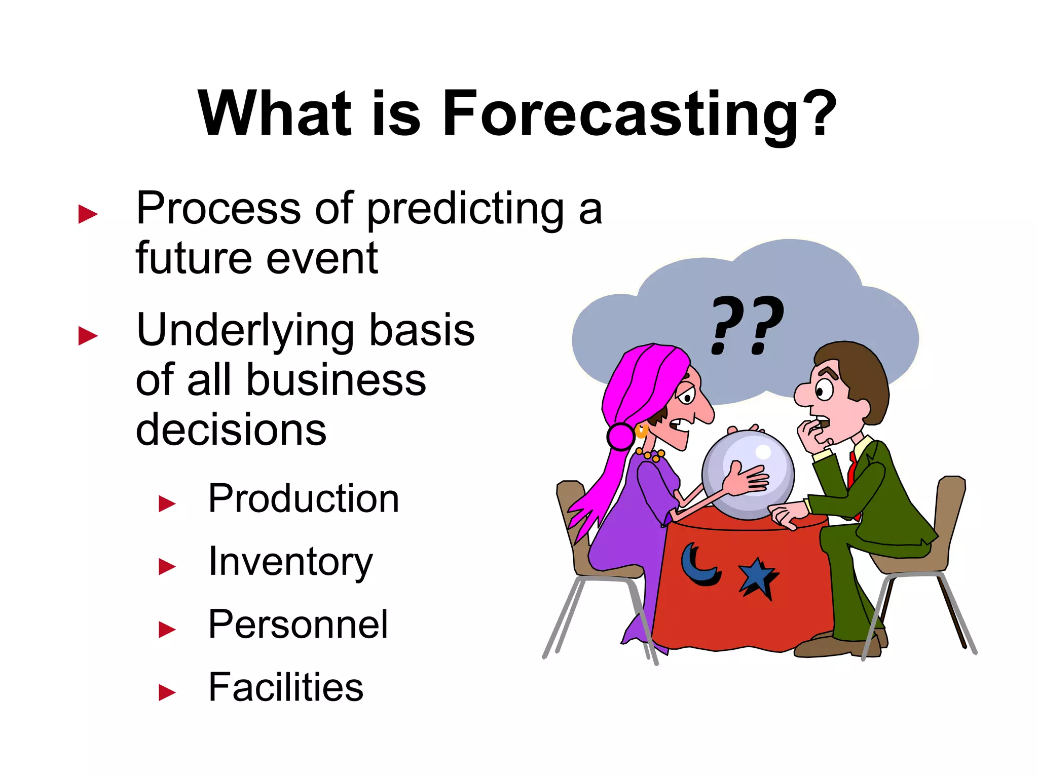
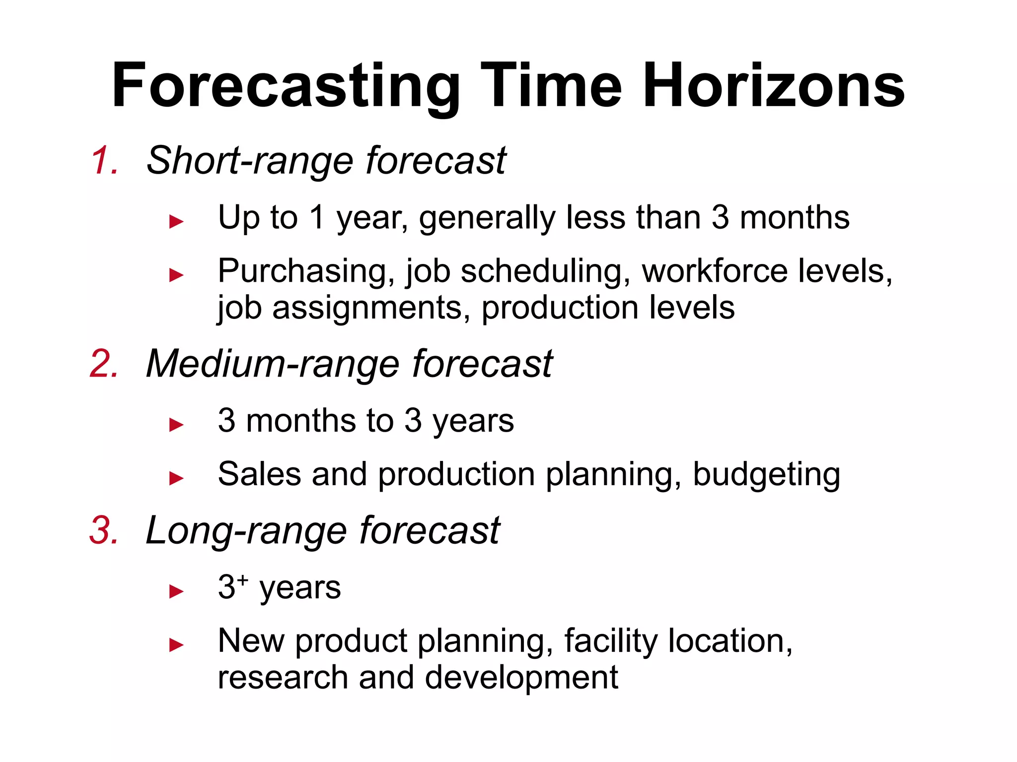
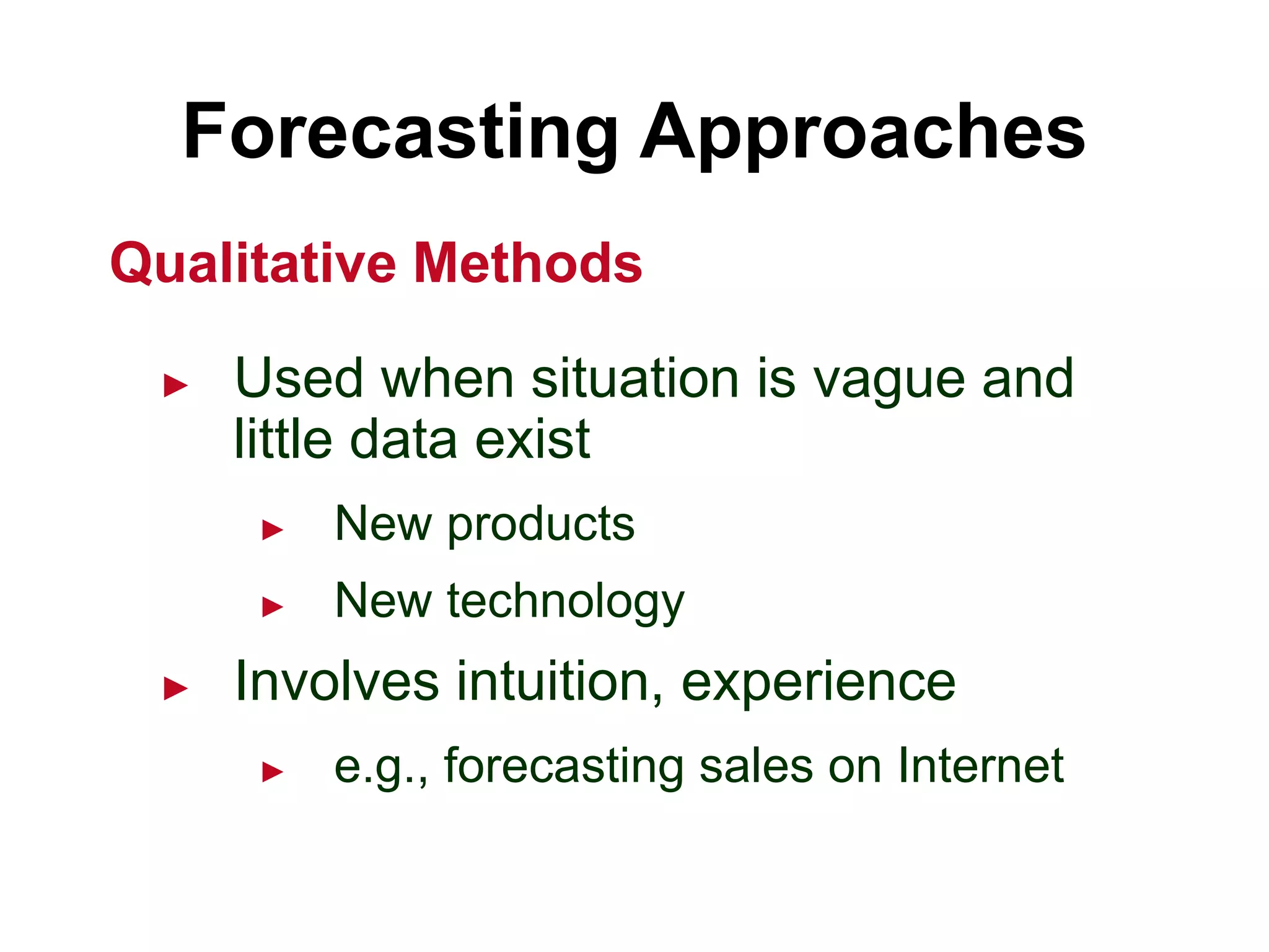
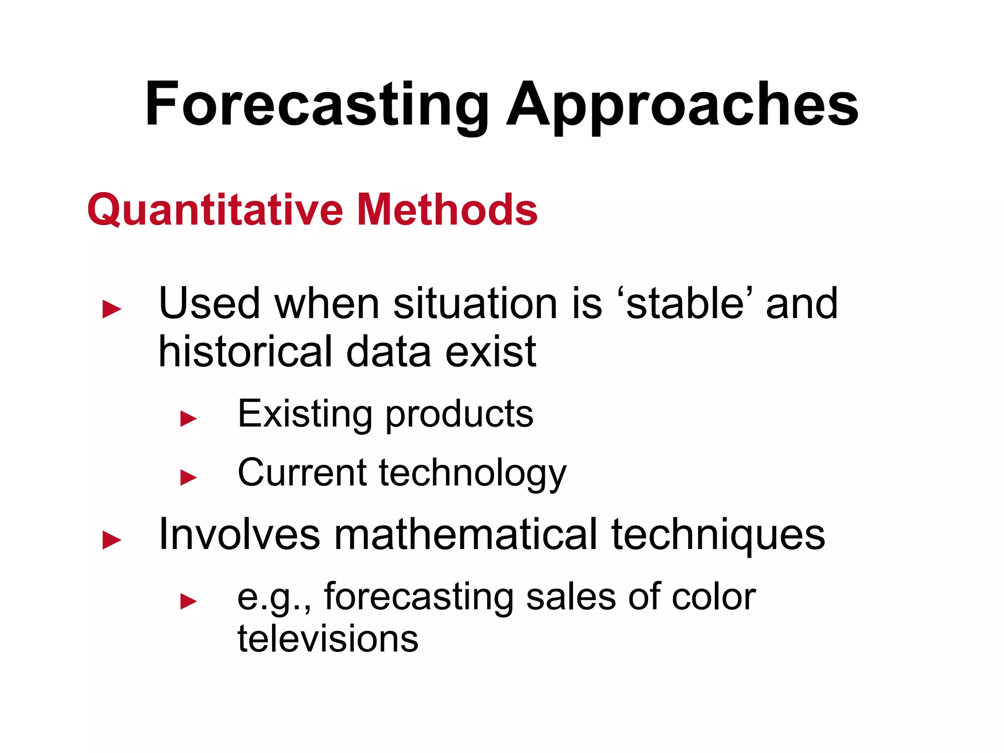
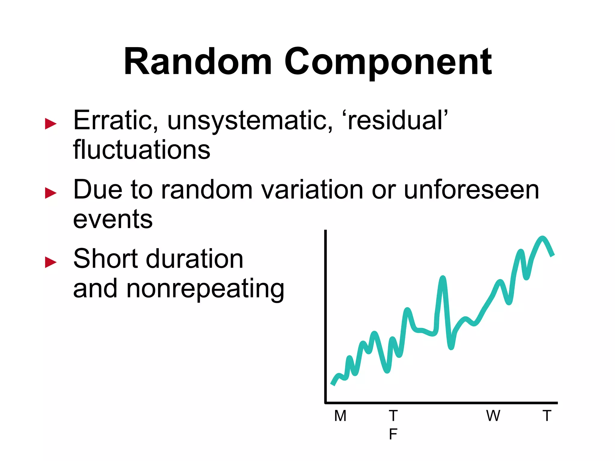
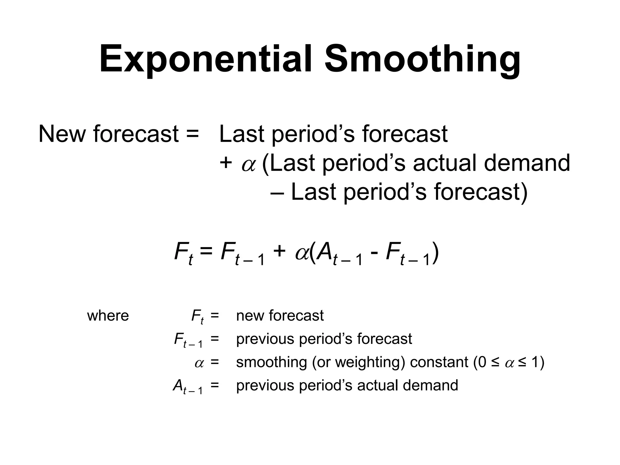
This document discusses forecasting methods. It defines forecasting as predicting future events and notes that forecasting underlies business decisions regarding production, inventory, personnel and facilities. It outlines different forecasting time horizons from short-range up to one year to long-range over three years. The document also discusses qualitative and quantitative forecasting approaches and provides examples of specific forecasting techniques like moving averages, exponential smoothing and error measurement methods.


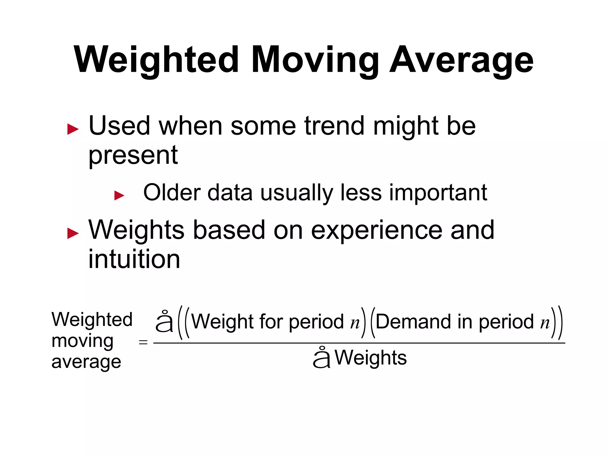
![Weighted Moving Average
MONTH ACTUAL SHED SALES 3-MONTH WEIGHTED MOVING AVERAGE
January 10
February 12
March 13
April 16
May 19
June 23
July 26
August 30
September 28
October 18
November 16
December 14
WEIGHTS APPLIED PERIOD
3 Last month
2 Two months ago
1 Three months ago
6 Sum of the weights
Forecast for this month =
3 x Sales last mo. + 2 x Sales 2 mos. ago + 1 x Sales 3 mos. ago
Sum of the weights
[(3 x 13) + (2 x 12) + (10)]/6 = 12 1/6
10
12
13](https://image.slidesharecdn.com/forecasting-180721091808/75/Forecasting-29-2048.jpg)
![Weighted Moving Average
MONTH ACTUAL SHED SALES 3-MONTH WEIGHTED MOVING AVERAGE
January 10
February 12
March 13
April 16
May 19
June 23
July 26
August 30
September 28
October 18
November 16
December 14
[(3 x 13) + (2 x 12) + (10)]/6 = 12 1/6
10
12
13
[(3 x 16) + (2 x 13) + (12)]/6 = 14 1/3
[(3 x 19) + (2 x 16) + (13)]/6 = 17
[(3 x 23) + (2 x 19) + (16)]/6 = 20 1/2
[(3 x 26) + (2 x 23) + (19)]/6 = 23 5/6
[(3 x 30) + (2 x 26) + (23)]/6 = 27 1/2
[(3 x 28) + (2 x 30) + (26)]/6 = 28 1/3
[(3 x 18) + (2 x 28) + (30)]/6 = 23 1/3
[(3 x 16) + (2 x 18) + (28)]/6 = 18 2/3](https://image.slidesharecdn.com/forecasting-180721091808/75/Forecasting-30-2048.jpg)


![Product1 [3] forecasting v2](https://cdn.slidesharecdn.com/ss_thumbnails/product13-forecastingv2-190226041012-thumbnail.jpg?width=640&height=640&fit=bounds)


