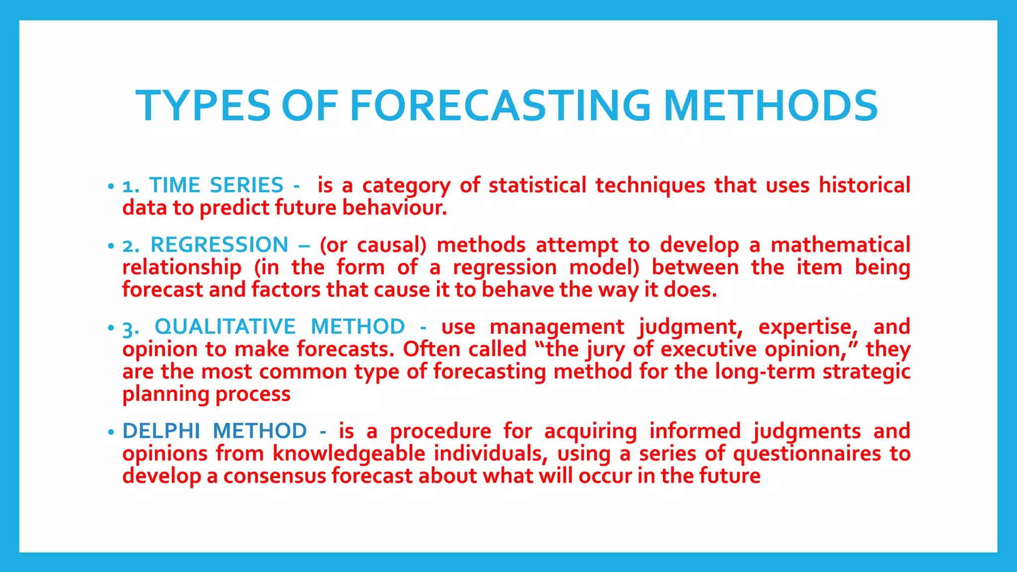
This document discusses forecasting methods used in agribusiness. It defines forecasting as predicting what will occur in the future, such as meteorologists forecasting weather or managers forecasting product demand. There are three main components of forecasting: time frame, existence of patterns, and number of variables. Time frames can be short-term, medium-term, or long-term. Forecasts often exhibit patterns like trends, cycles, or seasons. Common forecasting methods include time series analysis, regression, and qualitative techniques. Specific time series methods covered are moving averages, weighted moving averages, and exponential smoothing.

1. FORECASTINGAgribusiness 4
INTRODUCTIONTO MANAGEMENT SCIENCE
ARIES CUPASTIBAR
Instructor
Laguna State Polytechnic University

2. FORECASTING is a prediction of what will occur in the future.
METEOROLOGISTS - forecast the weather
SPORTS CASTERS - predict the winners
MANAGERS - predict how much of their
product will be demanded in the future.
FORECASTING COMPONENTS
FORECASTING METHOD
 time frame of the forecast
(how far in the future we are forecasting)
 existence of patterns in the forecast
(seasonal trends, peak periods)
 number of variables to which the forecast is related

3. CLASSIFICATION OFTIME FRAMES
• 1. Short-range forecasts - typically encompass the immediate future and are
concerned with the daily operations of a business firm, such as daily demand or
resource requirements.
• 2. Medium-range forecast - typically encompasses anywhere from 1 or 2 months
to 1 year. A forecast of this length is generally more closely related to a yearly
production plan and will reflect such items as peaks and valleys in demand and the
necessity to secure additional resources for the upcoming year
• 3. Long-range forecast - typically encompasses a period longer than 1 or 2 years.
Long-range forecasts are related to management’s attempt to plan new products
for changing markets, build new facilities, or secure long-term financing.
DAILY OPERATION
USUALLY FROM A MONTH UPTO AYEAR
MORE STRATEGIC AND FOR OVER AYEAR

4. Forecast often exhibit patterns, orTREND
• A trend is a long-term movement of the item being forecast.
For example, the demand for
personal computers has shown an
upward trend during the past
decade, without any long
downward movement in the
market. Trends are the easiest
patterns of demand behaviour to
detect and are often the starting
point for developing a forecast

5. Forecast often exhibit CYCLE
A cycle is an undulating movement in demand, up and down, that repeats itself
over a lengthy time span (i.e., more than 1 year).
For example, new housing
starts and thus construction-
related products tend to follow
cycles in the economy.
Automobile sales tend to follow
cycles in the same fashion. The
demand for winter sports
equipment increases every 4
years, before and after the
Winter Olympics.

6. Forecast often exhibit a SEASONAL PATTERN
A seasonal pattern is an oscillating movement in demand that occurs
periodically (in the short run) and is repetitive
For example, every December the
demand for toys and sketchers increases
dramatically, and retail sales in general
increase during the Christmas season
However, a seasonal pattern can occur
on a daily or weekly basis. For example,
some restaurants are busier at lunch
than at dinner, and shopping mall
stores and theatres tend to have higher
demand on weekends.

7. TYPES OF FORECASTING METHODS
• 1. TIME SERIES - is a category of statistical techniques that uses historical
data to predict future behaviour.
• 2. REGRESSION – (or causal) methods attempt to develop a mathematical
relationship (in the form of a regression model) between the item being
forecast and factors that cause it to behave the way it does.
• 3. QUALITATIVE METHOD - use management judgment, expertise, and
opinion to make forecasts. Often called “the jury of executive opinion,” they
are the most common type of forecasting method for the long-term strategic
planning process
• DELPHI METHOD - is a procedure for acquiring informed judgments and
opinions from knowledgeable individuals, using a series of questionnaires to
develop a consensus forecast about what will occur in the future

8. Time Series Methods
• 1. MOVING AVERAGE
• A time series forecast can be as simple as using demand in the
current period to predict demand in the next period.
For example, if demand is 100 units this week, the forecast for
next week’s demand would be 100 units; if demand turned out
to be 90 units instead, then the following week’s demand
would be 90 units, and so forth. This is sometimes referred to
as naïve forecasting. However, this type of forecasting method
does not take into account any type of historical demand
behaviour; it relies only on demand in the current period. As
such, it reacts directly to the normal, random up-and-down
movements in demand.

9. MOVING AVERAGE
• uses several values during the recent past to develop a
forecast.This tends to dampen, or smooth out, the random
increases and decreases of a forecast that uses only one
period
Moving averages are computed for specific periods, such as 3
months or 5 months, depending on how much the forecaster
desires to smooth the data.The longer the moving average
period, the smoother the data will be.

10. FORMULA: MOVING AVERAGE METHOD
MAn = 𝔦−1
𝔫
D𝔦
n
Where:
n = number of periods in the moving average
Di = data in period i

11. EXAMPLE:
MONTH ORDERS PER MONTH
JAN 120
FEB 90
MARCH 100
APRIL 75
MAY 110
JUN 50
JUL 75
AUG 130
SEPT 110
OCT 90
The Mushroom Production in LSPU sells and delivers Fresh Mushroom to various faculties, schools, and students
within a 30-mile radius of its area of production. Dr. Viyar wants to be certain that enough drivers and delivery
vehicles are available so that orders can be delivered promptly. Therefore, the manager wants to be able to
forecast the number of orders (kg.) that will occur during the next month (i.e., to forecast the demand for
deliveries).
The moving average forecast is computed by dividing the sum
of the values of the forecast variable, orders per month for a
sequence of months, by the number of months in the
sequence. Frequently, a moving average is calculated for three
or five time periods.
MAn = 𝔦−1
𝔫
D𝔦
n
MA3 = 𝐢−𝟏
𝟑
𝑫𝒊
3
= 90 + 110 + 130
3
= 330
3
= 110
orders3 MONTHS AVERAGE

12. MONTH ORDERS PER MONTH
JAN 120
FEB 90
MARCH 100
APRIL 75
MAY 110
JUN 50
JUL 75
AUG 130
SEPT 110
OCT 90
5 MONTHS AVERAGE
MAn = 𝔦−1
𝔫
D𝔦
n
= 90 + 110 + 130 + 75 + 50
5
= 445
5
= 91 orders

13. 3-and-5 MONTH AVERAGES
MONTH ORDERS PER MONTH
JAN 120
FEB 90
MARCH 100
APRIL 75
MAY 110
JUN 50
JUL 75
AUG 130
SEPT 110
OCT 90
NOV __________
3 – MONTH MOVING AVERAGE 5 – MONTH MOVING AVERAGE
________ ________
________ ________
________ ________
103.3 ________
88.3 ________
95.0 99.0
78.3 85.0
78.3 82.0
85.0 88.0
105.0 95.0
110.0 91.0

14. 120
90
100
75
110
50
75
130
110
90
99
85
82
88
95
0
20
40
60
80
100
120
140
1 2 3 4 5 6 7 8 9 10
VALUE
TIME
Forecasting
Demand Forecast
120
90
100
75
110
50
75
130
110
90
99
85
82
88
95
0
20
40
60
80
100
120
140
1 2 3 4 5 6 7 8 9 10
VALUE
TIME
Forecasting
Demand Forecast
3 MONTH 5 MONTH
FORECASTFORECAST
ACTUAL ACTUAL

15. Weighted Moving Average
• The moving average method can be adjusted to reflect more closely
more recent fluctuations in the data and seasonal effects. This
adjusted method is referred to as a weighted moving average
method. In this method, weights are assigned to the most recent
data according to the following formula:
WMAn = 𝑖−1
𝔫
𝑊𝑖𝐷𝑖
n
Where:
n = the weighted for periods, between 0% and 100% (i.e.
between o and 1.0
∑Wi = 1.0

16. EXAMPLE:
• For example, if the Dr. Viyar wants to compute a 3-month weighted
moving average with a weight of 50% for the October data, a weight of
33% for the September data, and a weight of 17% for August, it is
computed as
WMA3 = 𝑖−1
3
𝑊𝑖𝐷𝑖
n
= (0.50) (90) + (0.33) (110) + (0.17) (130)
MONTH ORDERS PER MONTH
JAN 120
FEB 90
MARCH 100
APRIL 75
MAY 110
JUN 50
JUL 75
AUG 130
SEPT 110
OCT 90
= 45 + 36.3 + 22.1
= 103.4 orders

17. EXPONENTIAL SMOOTHING
• The exponential smoothing forecast method is an averaging
method that weights the most recent past data more strongly
than more distant past data.
TWO FORMS OF EXPONENTIAL SMOOTHING:
1. Simple Exponential Smoothing
2. Adjusted Exponential Smoothing

18. • To demonstrate simple exponential smoothing, we will return
to the Mushroom Production in LSPU example. The simple
exponential smoothing forecast is computed by using the
formula:
Ft+1 = αDt + (1- α) Ft
Where: Ft+1 = the forecast for the next period
Dt = actual demand in the present period
Ft =the previously determined forecast for the present period
α = a weighting factor referred to as the smoothing constant
The smoothing constant, is between zero and one. It reflects the
weight given to the most recent demand data. For example,
if = α.20, Ft+1 = .20Dt + .80Ft

19. EXAMPLE:
Tibar’s Computer Services assembles customized personal
computers from generic parts. The company was formed and is
operated by two regular instructor in LSPU, Dr. Editha Perey and
Prof. Charmyne Sanglay, and has had steady growth since it
started. The company assembles computers mostly at night,
using other part-time instructor as labor. Dr. Perey and Prof.
Sanglay purchase generic computer parts in volume at a discount
from a variety of sources whenever they see a good deal. It is
therefore important that they develop a good forecast of demand
for their computers so that they will know how many computer
component parts to purchase and stock.

20. The company has accumulated the demand data for its computers
for the past 12 months, from which it wants to compute
exponential smoothing forecasts, using smoothing constants
equal to .30 and .50. PERIOD MONTH DEMAND Ft+1 =.3
1 JAN 37
2 FEB 40 37
3 MAR 41 37.9
4 APR 37 38.83
5 MAY 45 38.28
6 JUN 50
7 JUL 43
8 AUG 47
9 SEP 56
10 OCT 52
11 NOV 55
12 DEC 54
F2 = αD1 + (1 - α )F1
= (.30)(37) + (.70)(37)
= 37 units
F3 = αD2 + (1 - α )F2
= (.30)(40) + (.70)(37)
= 37.9 units
F4 = αD3 + (1 - α )F3
= (.30)(41) + (.70)(37.9)
= 38.83 units
F5 = αD4 + (1 - α )F4
= (.30)(37) + (.70)(38.83)
= 38.28 units

21. PERIOD MONTH DEMAND Ft+1 =.3 Ft+1 =.5
1 JAN 37 ------
2 FEB 40 37 37
3 MAR 41 37.9 38.5
4 APR 37 38.83 39.75
5 MAY 45 38.28 38.37
6 JUN 50 40.29 41.68
7 JUL 43 43.20
8 AUG 47 43.14
9 SEP 56 44.30
10 OCT 52 47.81
11 NOV 55 49.06
12 DEC 54 50.84
13 JAN ------ 51.79
α = .5
F2 = αD1 + (1 - α )F1
= (.5)(37) + (.5)(37)
= 37 units
F3 = αD2 + (1 - α )F2
= (.5)(40) + (.5)(37)
= 38.5 units
F4 = αD3 + (1 - α )F3
= (.5)(41) + (.5)(38.5)
= 39.75 units
F5 = αD4 + (1 - α )F4
= (.5)(37) + (.5)(39.75)
= 38.37 units
F6 = αD5 + (1 - α )F5
= (.5)(45) + (.5)(38.37)
= 41.68 units

22. PERIOD MONTH DEMAND Ft+1 =.3 Ft+1 =.5
1 JAN 37 ------
2 FEB 40 37 37
3 MAR 41 37.9 38.5
4 APR 37 38.83 39.75
5 MAY 45 38.28 38.37
6 JUN 50 40.29 41.68
7 JUL 43 43.20 45.84
8 AUG 47 43.14 44.42
9 SEP 56 44.30 45.71
10 OCT 52 47.81 50.85
11 NOV 55 49.06 51.42
12 DEC 54 50.84 53.21
13 JAN ------ 51.79 53.61
Based on simple observation of the two
forecasts in table (α=0.5), seems to be
the more accurate of the two, in the
sense that it seems to follow the actual
data more closely.
In general, when demand is relatively
stable, without any trend, using a small
value for is more appropriate to simply
smooth out the forecast. Alternatively,
when actual demand displays an
increasing (or decreasing) trend, as is the
case in our example, a larger value of is
generally better.

23. ADJUSTED EXPONENTIAL SMOOTHING
The adjusted exponential smoothing forecast
consists of the exponential smoothing forecast with a
trend adjustment factor added to it.
The formula for the adjusted forecast is
AFt+1 = Ft+1 +Tt+1
Where:
Tt+1 - an exponentially smoothed trend factor

24. The trend factor is computed much the same as the
exponentially smoothed forecast. It is, in effect, a forecast
model for trend:
Tt+1 = β(Ft+1 –Ft) + (1- β)Tt
Where:
Tt = the last period trend factor
β = a smoothing constant for trend

25. PERIOD MONTH DEMAND Ft+1
=.3
Ft+1
=.5
T
(Tt+1)
1 JAN 37 ------
2 FEB 40 37 37 0
3 MAR 41 37.9 38.5 0.45
4 APR 37 38.83 39.75 0.69
5 MAY 45 38.28 38.37
6 JUN 50 40.29 41.68
7 JUL 43 43.20 45.84
8 AUG 47 43.14 44.42
9 SEP 56 44.30 45.71
10 OCT 52 47.81 50.85
11 NOV 55 49.06 51.42
12 DEC 54 50.84 53.21
13 JAN ------ 51.79 53.61
Tt+1 = β(Ft+1 –Ft) + (1- β)Tt
T3 = β (F3-F2) + (1- β)T2
= 0.30(38.5-37) + 0.70(0)
= 0.30(1.5) + 0
= 0.45
T4= β (F4-F3) + (1- β)T3
= 0.30(39.75-38.5) + 0.70(0.45)
= 0.30(1.25) + 0.315
= 0.375 + 0.315
= 0.69

26. PERIOD MONTH DEMAND Ft+1
=.3
Ft+1
=.5
T
(Tt+1)
1 JAN 37 ------
2 FEB 40 37 37 0
3 MAR 41 37.9 38.5 0.45
4 APR 37 38.83 39.75 0.69
5 MAY 45 38.28 38.37 0.07
6 JUN 50 40.29 41.68 1.04
7 JUL 43 43.20 45.84 1.97
8 AUG 47 43.14 44.42 0.95
9 SEP 56 44.30 45.71 1.05
10 OCT 52 47.81 50.85 2.28
11 NOV 55 49.06 51.42 1.76
12 DEC 54 50.84 53.21 1.77
13 JAN ------ 51.79 53.61 1.36
T5 = β (F5-F4) + (1- β)T4
= 0.30(38.37-39.75) + 0.70(0.69)
= 0.30(-1.38) + 0.483
= -0.414+0.483
= 0.069 or 0.07
T6= β (F6-F5) + (1- β)T5
= 0.30(41.68-38.37) + 0.70(0.07)
= 0.30(3.31) + 0.049
= 0.993 + 0.049
= 1.042 or 1.04

27. PERIOD MONTH DEMAND Ft+1
=.3
Ft+1
=.5
T
(Tt+1)
ADJUSTED
Forecast
1 JAN 37 ------ -------- --------- -----------
2 FEB 40 37 37 0 37
3 MAR 41 37.9 38.5 0.45 38.95
4 APR 37 38.83 39.75 0.69 40.44
5 MAY 45 38.28 38.37 0.07 38.44
6 JUN 50 40.29 41.68 1.04 42.73
7 JUL 43 43.20 45.84 1.97 47.82
8 AUG 47 43.14 44.42 0.95 45.37
9 SEP 56 44.30 45.71 1.05 46.76
10 OCT 52 47.81 50.85 2.28 53.13
11 NOV 55 49.06 51.42 1.76 53.19
12 DEC 54 50.84 53.21 1.77 54.98
13 JAN ------ 51.79 53.61 1.36 54.96
AFt+1 = Ft+1 +Tt+1
AF2 = Ft+2 + Tt+2
= 37 + 0
= 37
AF3 = Ft+3 + Tt+3
= 38.5 + 0.45
= 38.95
AF4 = Ft+4 + Tt+4
= 39.75 + 0.69
= 40.44
˖ =

28. Regression Methods
Regression is a forecasting technique that measures
the relationship of one variable to one or more other
variables.
The simplest form of regression is linear regression,
which you will recall we used previously to develop a
linear trend line for forecasting.

29. Linear Regression
Simple linear regression relates one dependent variable to one
independent variable in the form of a linear equation:
𝒚 = 𝒂 + 𝒃𝒙
dependent variable independent variable
intercept slope

30. To develop the linear equation, the slope, b, and the
intercept, a, must first be computed by using the
following least squares formulas:
a = ӯ – bx
b= ∑xy -nẋӯ
∑x₂ - nẋ₂
Where:
x bar = sum of x data over no. of observations
y bar = sum of y data over no. of observations

31. EXAMPLE:
The BSAB Society wants to develop its budget for the coming year (2017),
using a forecast for the number of students enrolled. The Society Adviser
believes that the number of students enrolled in the program has directly
related to the funds that will be collected. The Society Adviser has
accumulated total annual number of students enrolled for the past 8 years:
YEAR FUNDS NUMBER OF STUDENTS
ENROLLED
1 26650 533
2 33700 674
3 33350 667
4 38250 765
5 43800 876
6 44500 890
7 45400 908
8 54900 1098

32. YEAR FUNDS
(x)
NUMBER OF
STUDENTS
ENROLLED (y)
xy x square
1 26650 533 14204450 284089
2 33700 674 22713800 454276
3 33350 667 22244450 444889
4 38250 765 29261250 585225
5 43800 876 38368800 767376
6 44500 890 39605000 792100
7 45400 908 41223200 824464
8 54900 1098 60280200 1205604
∑y=320550 ∑x= 6411 267901150 5358023
Given the number of students enrolled, the BSAB Adviser believes the Program will
get at least 1,200 next year. She wants to develop a simple regression equation for
these data to forecast funds to be collected for this level of success. The
computations necessary to compute a and b, using the least squares formulas, are
summarized inTable