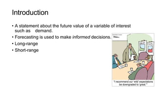
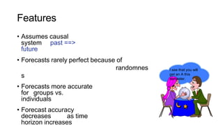
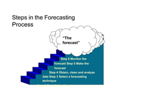
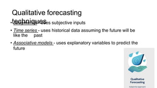
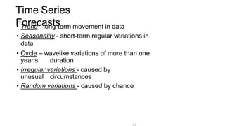
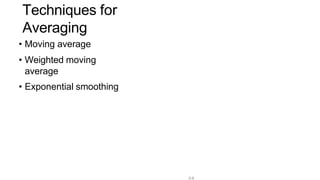
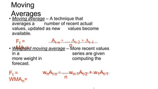
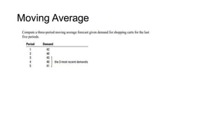
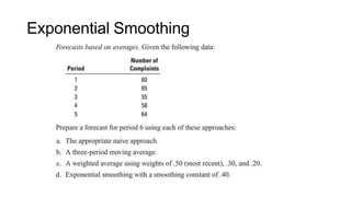
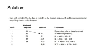
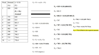
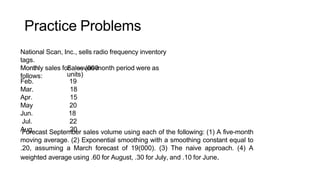
Demand forecasting involves predicting future demand based on historical data and various forecasting techniques such as judgmental, time series, and associative models. Different methods like moving averages and exponential smoothing are utilized to enhance accuracy, taking into account factors like trends, seasonality, and irregular variations. The document outlines a structured forecasting process and includes practices for calculating forecasts using specific data sets.

1. Demand
Forecasting

2. Introduction
• A statement about the future value of a variable of interest
such as demand.
• Forecasting is used to make informed decisions.
• Long-range
• Short-range

3. Features
• Assumes causal
system past ==>
future
• Forecasts rarely perfect because of
randomnes
s
• Forecasts more accurate
for groups vs.
individuals
• Forecast accuracy
decreases as time
horizon increases
I see that you will
get an A this
semester.

4. Elements of Forecasting
Timel
y
Accura
te
Reliabl
e
Writte
n

5. Steps in the Forecasting
Process
Step 6 Monitor the
forecast Step 5 Make the
forecast
Step 4 Obtain, clean and analyze
data Step 3 Select a forecasting
technique
Step 2 Establish a time
“The
forecast”

6. Qualitative forecasting
techniques
• Judgmental - uses subjective inputs
• Time series - uses historical data assuming the future will be
like the past
• Associative models - uses explanatory variables to predict the
future

7. 3-7
Judgmental
Forecasts
• Executive opinions- long range planning and
new product development
• Sales force opinions
• Consumer surveys
• Delphi method
• Opinions of managers and staff
• Achieves a consensus forecast

8. 3-8
Time Series
Forecasts
• Trend - long-term movement in data
• Seasonality - short-term regular variations in
data
• Cycle – wavelike variations of more than one
year’s duration
• Irregular variations - caused by
unusual circumstances
• Random variations - caused by chance

9. 3-9
Techniques for
Averaging
• Moving average
• Weighted moving
average
• Exponential smoothing

10. 3-
Moving
Averages
Ft =
MAn=
• Moving average – A technique that
averages a number of recent actual
values, updated as new values become
available.
At-n + … At-2 + At-1
n
Ft =
WMAn=
• Weighted moving average – More recent values
in a series are given
more weight in computing the
forecast.
wnAt-n + … wn-1At-2 + w1At-1
n

11. Moving Average

12. Solution

13. Weighted Moving Average

14. Solution

15. 3-
Exponential
Smoothing
Ft =Ft-1 + (At-1 - Ft-1)
• Premise--The most recent observations might
have the highest predictive value.
• Therefore, we should give more weight to the more
recent time periods when forecasting.

16. Exponential Smoothing

19. Solution

22. Practice Problems
National Scan, Inc., sells radio frequency inventory
tags.
Monthly sales for a seven-month period were as
follows:
Month Sales (000
units)
Feb. 19
Mar. 18
Apr. 15
May 20
Jun. 18
Jul. 22
Aug. 20
Forecast September sales volume using each of the following: (1) A five-month
moving average. (2) Exponential smoothing with a smoothing constant equal to
.20, assuming a March forecast of 19(000). (3) The naive approach. (4) A
weighted average using .60 for August, .30 for July, and .10 for June.

23. An electrical contractor’s records during the last five weeks
indicate the number of job requests:
Week: 1 2 3 4 5
Requests: 20 22 18 21 22
Predict the number of requests for week 6 using each of these
methods:
a. Naive. b. A four-period moving average. c. Exponential
smoothing with
0.30. Use 20 for week 2 forecast.