Rolle's theorem states that if a function is continuous on a closed interval and differentiable on the open interval with equal values at the endpoints, then the derivative is 0 for at least one value in the interval. The mean value theorems - Lagrange's and Cauchy's - generalize this idea, relating the average rate of change over an interval to the instantaneous rate at a point within the interval. Examples are provided to illustrate the theorems and exceptions that can occur when their conditions are not fully met.

1. Rolle’s Theorem
Statement
Let a function f:[a,b]R be such that
(i) f is continuous on [a,b],
(ii) f is differentiable on (a,b), and
(iii) f(a)=f(b).
Then there exists at least one point c(a,b) such that f )=0.
If f crosses the axis twice, somewhere between the two
crossings, the function is flat. The accurate statement of this
``obvious'' observation is Rolle's Theorem.

2. Interpretation of Rolle’s Theorem
Geometrical Interpretation:
If the function y=f(x) has a graph which is a continuous curve on
[a,b], and the curve has a tangent at every point of (a,b), and
f(a)=f(b), then there must exist at least one point c in (a,b) such that
the tangent to the curve at (c,f(c)) is parallel to the x-axis.

3. Algebraic interpretation:
If the function f(x) satisfies all the conditions of Rolle’s Theorem,
then between two zeros a and b of f(x) there exists at least one zero
of f (x) [i.e., between two roots a and b of f(x) =0 there must exist at
least one root of f (x)=0].
Immediate conclusion:
Between two consecutive roots of f (x)=0, there lies at most one root
of f(x)=0.
Important note:
The set of conditions in the Rolle’s Theorem is a set of sufficient
conditions.
The conditions are by no means necessary.
Illustrations:
i) The function f defined in [0,1] as follows:
f(x)=1, 0
=2, .
The function f(x) satisfies none of the conditions of Rolle’s
Theorem, yet f'(x)=0 for many points in [0,1].

4. ii) The function f defined in [-1,3] as follows:
f(x)= + .
The function f(x) satisfies none of the conditions of Rolle’s
Theorem, yet f'(x)=0 for many points in [-1,3],
In fact f'(x)=0 for all x(0,1).
The above two examples show that the conditions in the
Rolle’s Theorem are not absolute necessity for f'(x) to be
zero at some point in the concerned interval.
iii) The function f defined in [-1,1] as follows:
f(x)= .
Here,
f(x) is continuous on [-1,1],
f(-1)=f(1),
but f'(0) does not exists i.e. , f(x) is not differentiable on
(-1,1).
Also,
f'(x) vanishes nowhere in (-1,1)-{0}.
Failure of Rolle’s Theorem can be explained by the fact
that is not derivable in -1<x<1, though other
conditions are satisfied.
iv) The function f defined in [-1,1] as follows:
f(x)=x3+5x-4.
f(x) is continuous on [-1,1],
f(x) is derivable on (-1,1),
but f(-1)≠f(1).
Also,
f'(x) =3x2+5 vanishes nowhere in (-1,1).
Failure of Rolle’s Theorem can be explained by the fact
that , though other conditions are satisfied.

5. v) The function f defined in [-1,1] as follows:
f(x)=x2, x=-1
= 5x , -1<x<1
= x2, x=1
Here,
f(x) is continuous on (-1,1) and discontinuous at the points
x=-1 and x=1.
i.e., f(x) is not continuous on [-1,1],
f(x) is derivable on (-1,1),
and f(-1)=f(1).
f'(x) vanishes nowhere in (-1,1).
Failure of Rolle’s Theorem can be explained by the fact
that f(x) is not continuous in -1 1, though other
conditions are satisfied.
Examples (iii), (iv)& (v) show that if we drop any of the conditions in
Rolle’s Theorem then Rolle’s Theorem fails to be true.
Important Note:
If f(x) satisfies all the conditions of Rolle’s Theorem in
[a,b] then the conclusion that f (c)=0 where a<c<b is
assured, but if any of the conditions are violated then
Rolle’s Theorem will not be necessarily true; it may still
be true but the truth is not ensured.

6. Lagrange’s Mean Value Theorem
(First Mean Value Theorem of Differential Calculus)
Statement
Let a function f:[a,b]R be such that
i) f is continuous on [a,b],
ii) f is differentiable on (a,b).
Then there exists at least one point c(a,b) such that
Another Form of Lagrange’s MVT:
If in the statement of the theorem, b is replaced by a+h, (h>0), then
the number between a and b may be written as a+θh, where
0<θ<1.
Then the theorem takes the following form:
Let f:[a,a+h]R be such that
iii) f is continuous on [a,a+h],
iv) f is differentiable on (a,a+h).
Then there exists a real number θ lying between 0 and 1 such that

7. or, f(a+h)=f(a)+hf′(a+θh).
** Mean Value Theorem relates the mean rate of change
to instantaneous rate of the function.
Somewhere inside a chord, the tangent to f will be parallel to
the chord. The accurate statement of this common-sense
observation is the Mean Value Theorem

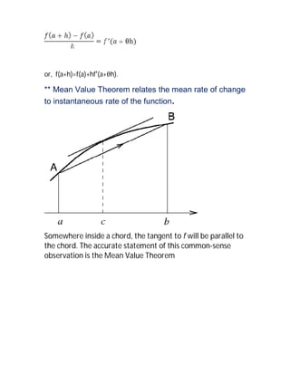
8. For any function that is continuous on [a, b] and differentiable
on (a, b) there exists some c in the interval (a, b) such that
the secant joining the endpoints of the interval [a, b] is
parallel to thetangent at c.
Geometrical Interpretation:
If the function y=f(x) has a graph which is a continuous curve on
[a,b], and the curve has a tangent at every point of (a,b),then there
exists at least one point c in (a,b) such that the tangent to the curve
at (c,f(c)) is parallel to the line segment joining the points (a,f(a)) and
(b,f(b)).
Remarks:
i) The fraction measures the mean (or average) rate of
increase of the function in the interval [a,b] of length b-a.
Hence the theorem expresses the fact that, under the
conditions stated, the mean rate of increase in any
interval [a,b] is equal to the actual rate of increase at

9. some point c within the interval (a,b). For instance, the
mean velocity of a moving car in any interval of time is
equal to the actual velocity at some instant within the
interval. This justifies the name Mean Value Theorem.
ii) Mean Value Theorem proposes that any differentiable function
defined over an interval has a mean value at which a
tangent line is parallel to the line joining the end points of
the function’s graph on that interval.
iii) Rolle’s Theorem is a particular case of Lagrange’s Mean Value
Theorem. If f(a)=f(b) holds in addition to the two
conditions of Mean Value Theorem then f(b)-f(a)=0 and
consequently f (c)=0.
Important deductions:
i) Let f:[a,b]R be such that
*f is continuous on [a,b],
*f is differentiable on (a,b)
And * f'(x)=0 for all x(a,b).
Then f(x) is a constant function on [a,b].
ii) Let f:[a,b]R be such that
*f is continuous on [a,b],
*f is differentiable on (a,b)
and * f'(x) 0 for all x(a,b).
Then f(x) is a monotone increasing function on [a,b].

10. iii) Let f:[a,b] R be such that
*f is continuous on [a,b],
*f is differentiable on (a,b)
and * f'(x) 0 for all x(a,b).
Then f(x) is a monotone decreasing function on [a,b].
Cauchy’s Mean Value Theorem:
(Second Mean Value Theorem of Differential Calculus)
Statement
Let the functions f:[a,b]R and g:[a,b]R be such that
i) both f,g are continuous on [a,b],
ii) both f,g are differentiable on (a,b), and
iii) f'(x)≠0 for x(a,b).
Then there exists at least one point (a,b) such that
.

11. Second Statement:
Let the functions f:[a,a+h]R and g:[a,a+h]R be such that
iv) both f,g are continuous on [a,a+h],
v) both f,g are differentiable on (a,a+h), and
vi) f'(x)≠0 for x(a,a+h).
Then there exists at least one real number θ lying between 0 and 1
such that
.
Geometric Interpretation of Cauchy’s
MVT:
First Interpretation: The functions f and g can considered as
determining a curve in the plane by means of parametric equations
x=f(t),y=g(t),where atb. Cauchy’s MVT concludes that  a point
(f(),g())of the curve for some t= in (a,b) such that the slope of the
line segment joining the end points (f(a),g(a)) and (f(b),g(b)) of the
curve is equal to the slope of the tangent to the curve at t=.

12. Second Interpretation: We may write
Hence, the ratio of the mean rates of increase of two functions in an
interval [a,b] is equal to the ratio of the actual rates of increases of
the functions at some point  within the interval (a,b).
REMARKS:
i) Lagrange’s MVT can be deduced from Cauchy’s MVT by taking
f(x)=x, x(a,b).
ii) Rolle’s Theorem can be obtained from Cauchy’s MVT by letting
f(x)=x and g(b)=g(a).
[We have used Rolle’s Theorem to prove Cauchy’s MVT.]

13. iii) Both f and g satisfy the conditions of Lagrange’s MVT.
Consequently there exist points c and d in (a,b) such that
and
c and d are different points in (a,b) in general, and
therefore a single point  in (a,b) may not be found to
satisfy the conclusion of Cauchy’s MVT.
Some problems:
Q1. Show that the equation 4x5+x3+7x-1=0 has exactly one
real root.
Q2. A function f is differentiable on [0,2] and
f(0)=0,f(1)=1,f(2)=1. Prove that f'(c)=0 for some c in (0,2).
Q3. Prove that the equation (x-1)3+(x-2)3+(x-3)3+(x-
4)3=0 has only one real root.
Q4. Prove that between any two real roots of excosx+1=0
there is at least one real root of exsinx+1=0.
Q5. Verify Lagrange’s MVT for the function f(x) =x(x-1)(x-2)
in the interval [0, ].
Q6. Show that
if 0<u<v
deduce that
< < .

14. Q7. If in the Cauchy’s MVT we take f(x)= and g(x)= ,
then prove that  is the arithmetic mean between a and b.
(Refer to the statement of Cauchy’s MVT).
Q8. If f(x)= (x-a)m(x-b)n where m and n are positive integers,
show that c in Rolle’s theorem divides the segment a x b in
the ratio m:n.
Q9. Apply MVT to prove that lies between 10 and
10.05.
Q10. Show that
, where 0< .