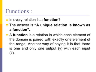
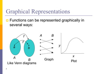
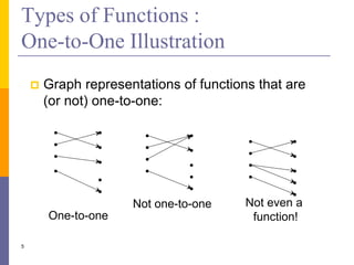
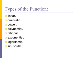
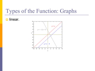
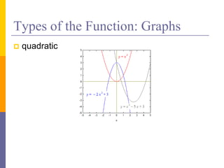
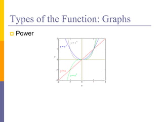
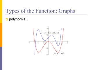
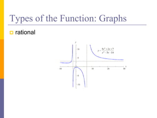
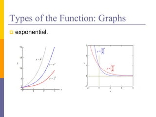
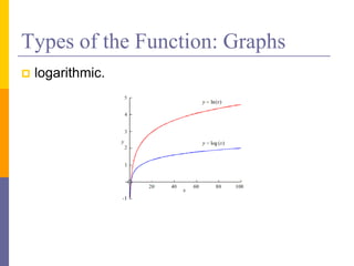
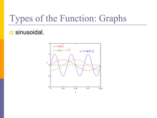
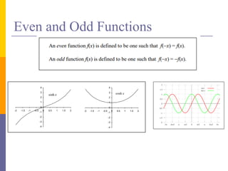
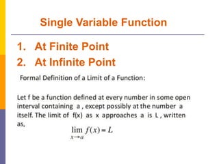
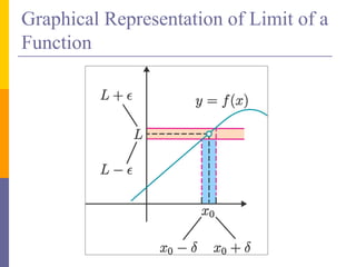
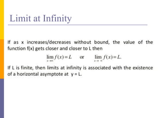
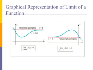
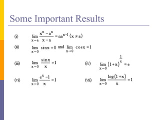
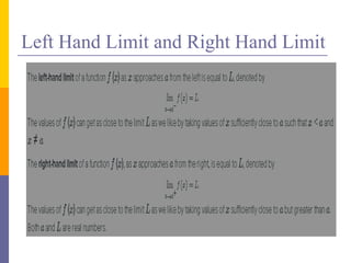
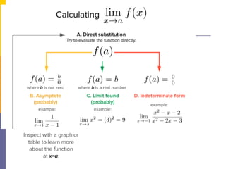
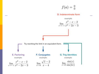
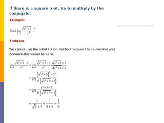
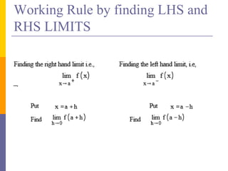
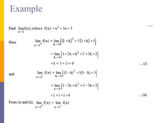
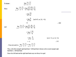
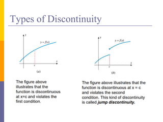
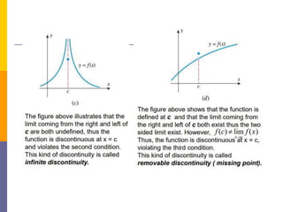
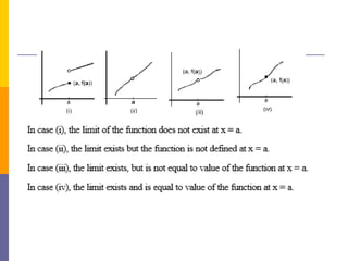
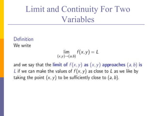
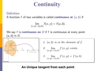
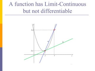
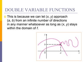
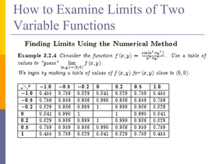
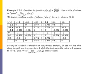
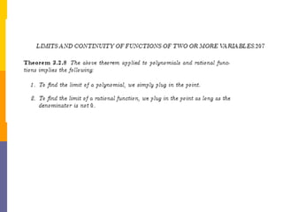
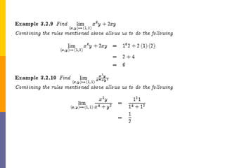
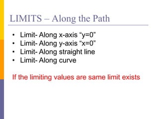
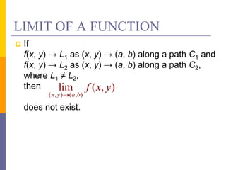
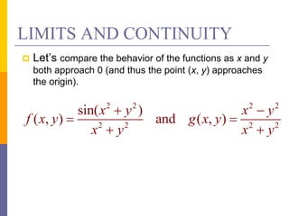
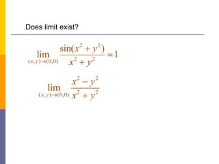
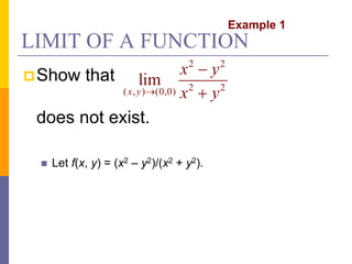
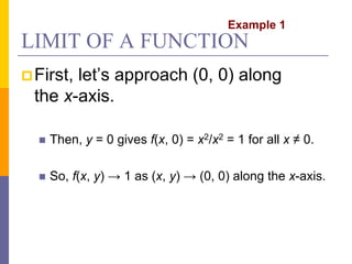
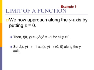
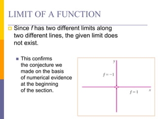
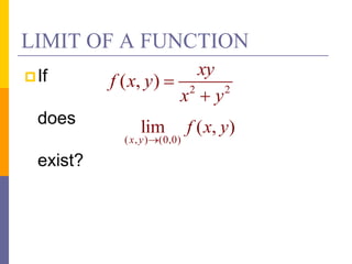
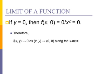
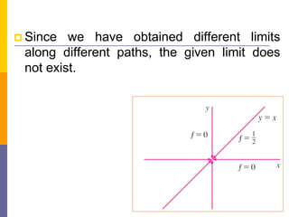
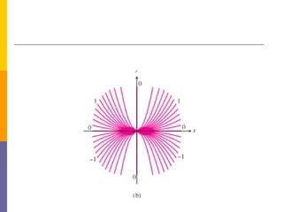
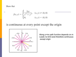
The document provides an overview of functions and limits. It defines a function as a relation where each input is paired with exactly one output. Functions can be represented graphically and include types like linear, quadratic, polynomial, and trigonometric. Limits describe the behavior of a function as inputs approach a value. For single-variable functions, limits can be evaluated at finite and infinite points. For multi-variable functions, limits may not exist if the function approaches different values along different paths to the point. Continuity requires a function's limit to exist and agree with its actual value at a point.

1. Lecture on Limits and
Continuity
Dr. Manisha Jain

2. Functions :
 Is every relation is a function?
 The answer is “A unique relation is known as
a function”.
 A function is a relation in which each element of
the domain is paired with exactly one element of
the range. Another way of saying it is that there
is one and only one output (y) with each input
(x).

3. 3
Graphical Representations
 Functions can be represented graphically in
several ways:
• •
A
B
a b
f
f
•
•
•
•
•
•
•
•
•
x
y
Plot
Graph
Like Venn diagrams
A B

4. 4
Some Function Terminology
 If f:AB, and f(a)=b (where aA & bB), then:
 A is the domain of f.
 B is the codomain of f.
 b is the image of a under f.
 a is a pre-image of b under f.
 In general, b may have more than one pre-image.

5. 5
Types of Functions :
One-to-One Illustration
 Graph representations of functions that are
(or not) one-to-one:
•
•
•
•
•
•
•
•
•
One-to-one
•
•
•
•
•
•
•
•
•
Not one-to-one
•
•
•
•
•
•
•
•
•
Not even a
function!

6. Types of the Function:
 linear.
 quadratic.
 power.
 polynomial.
 rational.
 exponential.
 logarithmic.
 sinusoidal.

7. Types of the Function: Graphs
 linear.

8. Types of the Function: Graphs
 quadratic

9. Types of the Function: Graphs
 Power

10. Types of the Function: Graphs
 polynomial.

11. Types of the Function: Graphs
 rational

12. Types of the Function: Graphs
 exponential.

13. Types of the Function: Graphs
 logarithmic.

14. Types of the Function: Graphs
 sinusoidal.

15. Implicit and Explicit Function
 IMPLICIT IS INDIRECT BUT
EXPLICIT IS DIRECT
 Explicit Function :
 Implicit Function :
2
0
y ax b
ax bx c
 
  
2 2
0
ax bxy cxy
  

16. Algebraic and Transcendental
Functions
 Algebraic Functions :
 Contains only Algebraic
Terms
 Transcendental
Function :
 Contains other
functions with
algebraic terms

17. Even and Odd Functions

18. Limits and Continuity

19. Limits of a Function
1. Single Variable Function
2. Two or more Variables

20. Single Variable Function
1. At Finite Point
2. At Infinite Point

21. Graphical Representation of Limit of a
Function

22. Limit at Infinity

23. Graphical Representation of Limit of a
Function

24. Theorems on Limits

25. Some Important Results

26. Left Hand Limit and Right Hand Limit

29. How to find Limits

34. Working Rule by finding LHS and
RHS LIMITS

35. Example

37. : ( ) 1; 7
Let f x x x
  
Limits – Numerically

38. At Infinite Point- Single Variable
 Try to get 1/ form so that the whole expression
will become zero

40. Some Examples on Piece Wise
Continuous Function

43. Types of Discontinuity

46. Limit and Continuity For Two
Variables

47. Continuity
An Unique tangent from each point

48. A function has Limit-Continuous
and differentiable

49. A function has Limit-Continuous
but not differentiable

50.  In general, we use the notation
 to indicate that:
 The values of f(x, y) approach the number L
as the point (x, y) approaches the point (a, b)
along any path that stays within the domain of f.
( , ) ( , )
lim ( , )
x y a b
f x y L



51. Notations for the limit :
lim ( , )
( , ) as ( , ) ( , )
x a
y b
f x y L
f x y L x y a b



 

52. Illustration of Definition

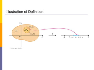
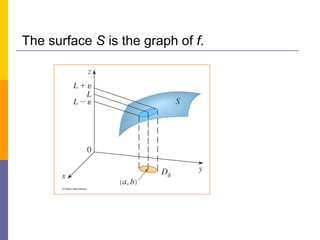
53.  If any small interval (L – ε, L + ε) is given around L, then
we can find a disk Dδ with center (a, b) and radius δ > 0
such that:
 f maps all the points in Dδ [except possibly (a, b)]
into the interval (L – ε, L + ε).

54. The surface S is the graph of f.

55. DOUBLE VARIABLE FUNCTIONS
 This is because we can let (x, y) approach
(a, b) from an infinite number of directions
in any manner whatsoever as long as (x, y) stays
within the domain of f.

56. How to Examine Limits of Two
Variable Functions

63. LIMITS – Along the Path
• Limit- Along x-axis “y=0”
• Limit- Along y-axis “x=0”
• Limit- Along straight line
• Limit- Along curve
If the limiting values are same limit exists

65. LIMIT OF A FUNCTION
 If
f(x, y) → L1 as (x, y) → (a, b) along a path C1 and
f(x, y) → L2 as (x, y) → (a, b) along a path C2,
where L1 ≠ L2,
then
does not exist.
( , ) ( , )
lim ( , )
x y a b
f x y


66. LIMITS AND CONTINUITY
 Let’s compare the behavior of the functions as x and y
both approach 0 (and thus the point (x, y) approaches
the origin).
2 2 2 2
2 2 2 2
sin( )
( , ) and ( , )
x y x y
f x y g x y
x y x y
 
 
 

67. Does limit exist?
2 2
2 2
( , ) (0,0)
sin( )
lim 1
x y
x y
x y




2 2
2 2
( , ) (0,0)
lim
x y
x y
x y




68. LIMIT OF A FUNCTION
Show that
does not exist.
 Let f(x, y) = (x2 – y2)/(x2 + y2).
Example 1
2 2
2 2
( , ) (0,0)
lim
x y
x y
x y




69. LIMIT OF A FUNCTION
First, let’s approach (0, 0) along
the x-axis.
 Then, y = 0 gives f(x, 0) = x2/x2 = 1 for all x ≠ 0.
 So, f(x, y) → 1 as (x, y) → (0, 0) along the x-axis.
Example 1

70. LIMIT OF A FUNCTION
We now approach along the y-axis by
putting x = 0.
 Then, f(0, y) = –y2/y2 = –1 for all y ≠ 0.
 So, f(x, y) → –1 as (x, y) → (0, 0) along the y-
axis.
Example 1

71. LIMIT OF A FUNCTION
 Since f has two different limits along
two different lines, the given limit does
not exist.
 This confirms
the conjecture we
made on the basis
of numerical evidence
at the beginning
of the section.

72. LIMIT OF A FUNCTION
If
does
exist?
2 2
( , )
xy
f x y
x y


( , ) (0,0)
lim ( , )
x y
f x y


73. LIMIT OF A FUNCTION
If y = 0, then f(x, 0) = 0/x2 = 0.
 Therefore,
f(x, y) → 0 as (x, y) → (0, 0) along the x-axis.

74. LIMIT OF A FUNCTION
If x = 0, then f(0, y) = 0/y2 = 0.
 So,
f(x, y) → 0 as (x, y) → (0, 0) along the y-axis.

75.  Let’s now approach (0, 0) along another line,
say y = x.
 For all x ≠ 0,
 Therefore,
2
2 2
1
( , )
2
x
f x x
x x
 

1
2
( , ) as ( , ) (0,0) along
f x y x y y x
  

76.  Since we have obtained different limits
along different paths, the given limit does
not exist.

77. Case-1: Value of the functions o various
paths
If
does
exist?
2
2 4
( , )
xy
f x y
x y


( , ) (0,0)
lim ( , )
x y
f x y


78.  Lets try to save time by letting (x, y) → (0, 0) along
any non-vertical line through the origin.: Then, y =
mx, where m is the slope,
and 2
2 4
2 3
2 4 4
2
4 2
( )
( , ) ( , );
( )
1
x mx
f x y f x mx
x mx
m x
x m x
m x
m x
 






79.  Therefore,
f(x, y) → 0 as (x, y) → (0, 0) along y = mx
 Thus, f has the same limiting value along
every non-vertical line through the origin.

80.  However, that does not show that the given limit is 0.
 This is because, if we now let (x, y) → (0, 0)
along the parabola x = y2
we have:
 So,
f(x, y) → ½ as (x, y) → (0, 0) along x = y2
2 2 4
2
2 2 4 4
1
( , ) ( , )
( ) 2 2
y y y
f x y f y y
y y y

   

Since different paths lead to different limiting
values, the given limit does not exist.

84. Along y=mx path function depends on m
Leads no limit exist therefore continuous
except origin