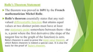
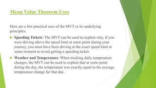
Rolle's theorem, proved by Michel Rolle in 1691, states that if a real-valued differentiable function has equal values at two distinct points, there is at least one stationary point between them where the derivative is zero. The theorem serves as a foundation for the Mean Value Theorem (MVT), which ensures that for continuous and differentiable functions, there exists a point where the instantaneous rate of change matches the average rate of change over an interval. Practical applications of these theorems include traffic management and financial modeling.

1. Rolle’s Theorem
M.Haseeb
22-NTU-CS-1860

2. Rolle’s Theorem Statement
 The theorem was proved in 1691 by the French
mathematician Michel Rolle.
 Rolle's theorem essentially states that any real-
valued differentiable function that attains equal
values at two distinct points must have at least
one stationary point somewhere between them—that
is, a point where the first derivative (the slope of the
tangent line to the graph of the function) is zero.
Rolle's theorem is used to prove the mean value theorem, of
which Rolle's theorem is indeed a special case. It is also the
basis for the proof of Taylor's theorem.

3. Geometrical Presentation of Rolle’s Theorem
Rolle's Theorem states the following:
 Suppose you have a real-valued function
f(x) that is continuous on a closed
interval[a , b].
 If f(x) is also differentiable on the open
interval (a , b), meaning it has a derivative
for every point between a and b, then
 If f(a)=f(b), meaning the function's values
at the endpoints of the interval are equal,
 Then there exists at least one point c in the
open interval (a , b) such that f'(c) = 0), in
other words, the derivative of the function
is zero at c.

4. Rolle’s Theorem Uses
The concept of Rolle's Theorem and related mathematical principles
can be indirectly applied:
 Traffic Control and Speed Limits: The concept of acceleration
and deceleration, which is fundamental in understanding calculus
and derivatives, plays a role in setting speed limits and designing
road systems to ensure safety. The analysis of changes in velocity
is based on principles related to calculus.
 Finance and Investments: Calculus concepts are often used in
modeling financial markets, predicting investment returns, and
managing risk. Derivatives, in particular, are essential in options
trading and risk management.

5. Example
The graph of f(x) = sin(x) + 2 for 0 ≤ x ≤ 2π is shown below.
f(0) = f(2π) = 2 and f is continuous on [0 , 2π] and
differentiable on (0 , 2π) hence, according to Rolle's
theorem, there exists at least one value ( there may be more
than one! ) of x = c such that f '(c) = 0.
f '(x) = cos(x)
f '(c) = cos(c) = 0
The above equation has two solutions on the interval [0 , 2π]
c 1 = π/2 and c 2 = 3π/2.
Therefore both at x = π/2 and x = 3 π/2 there are tangents to
the graph that have a slope equal to zero (horizontal line).

6. Mean Value Theorem Statement
The statement of the Mean Value Theorem is as follows:
 Mean Value Theorem (MVT):
Suppose f(x) is a real-valued function that is continuous on the
closed interval [a , b] and differentiable on the open interval (a
, b), where a<b. Then there exists at least one point c in the
open interval (a , b) such that:
 f′(c)=b−a f(b)−f(a)​

7. Geometrical presentation of Mean Value Theorem
 Consider a function f(x) that is continuous on the closed interval [ a ,b ]
and differentiable on the open interval (a , b).
 Plot the graph of f(x) on the coordinate plane. The function should be
continuous, meaning there are no jumps, gaps, or vertical asymptotes
within the interval [a , b].
 Draw a secant line between the points (a , f(a)) and(b ,f(b)). This secant
line represents the average rate of change of the function f(x) over the
interval [a , b].
 Now, according to the Mean Value Theorem, there must be at least one
point c in the open interval (a , b) where the tangent line (the
instantaneous rate of change) to the graph of f(x) is parallel to the secant
line.
 The slope of the secant line, which is b−a f(b)−f(a)​, is equal to the slope
of the tangent line at point c. Therefore, we have f′(c)=b−a f(b)−f(a)​.

8. Mean Value Theorem Uses
Here are a few practical uses of the MVT or its underlying
principles:
 Speeding Tickets: The MVT can be used to explain why, if you
were driving above the speed limit at some point during your
journey, you must have been driving at the exact speed limit at
some moment to avoid getting a speeding ticket.
 Weather and Temperature: When tracking daily temperature
changes, the MVT can be used to explain that at some point
during the day, the temperature was exactly equal to the average
temperature change for that day.

9. Example
Example : Verify Mean Value Theorem for the function f(x) = x2 + 1 in the interval [1, 4]. If so, find
the value of 'c'.
Solution:
The function is f(x) = x2 + 1. To verify the mean value theorem, the function f(x) = x2 + 1 must be
continuous in [1, 4] and differentiable in (1, 4).
Since f(x) is a polynomial function, both of the above conditions hold true.
The derivative f'(x) = 2x (power rule) is defined in the interval (1, 4)
f(1) = 12 + 1 = 1 + 1 = 2
f(4) = 42 + 1 = 16 + 1 = 17
f'(c) = [ f(4) - f(1) ] / (4 - 1)
= (17 - 2) / (4 - 1) = 15/3 = 5
f'(c) = 5
2c = 5
c = 2.5 which lies in the interval (1, 4)
Answer: Hence Mean Value Theorem is verified.