The document discusses various numerical computation methods for integrating and interpolating functions using MATLAB. It includes questions that assess knowledge on integration rules, error in interpolation, and MATLAB scripting related to evaluating functions and finding errors in approximations. The content emphasizes the importance of selecting appropriate numerical methods and understanding their accuracy.

1. Numerical Computation
Visit Us:
www.matlabassignmentexperts.com
Contact Us:
info@matlabassignmentexperts.com or,
Whatapp’s Us: +1 (315) 557-6473

2. Question 1. Consider the integral of a linear function,
in which α and β are any non-zero constants (e.g., α = 2, β = 4.5). We approximate this
by first breaking up the full interval into N − 1 segments of equal length h and then app
integration rule. Which of the following integration rules will yield the exact result for the
of equation (1) for any value of h?
(a) rectangle, left
(b) rectangle, right
(c) trapezoid
(d) rectangle, midpoint
Please circle all answers that apply. You will get full credit for circling all the correct ans
no incorrect answers, proportional partial credit for circling some of the correct answer(
and no incorrect answers, and zero credit if you circle any incorrect answers.
(Hint: Draw a simple picture.)
Question 2. The function f(x) is defined over the interval 0 ≤ x ≤ 1 by

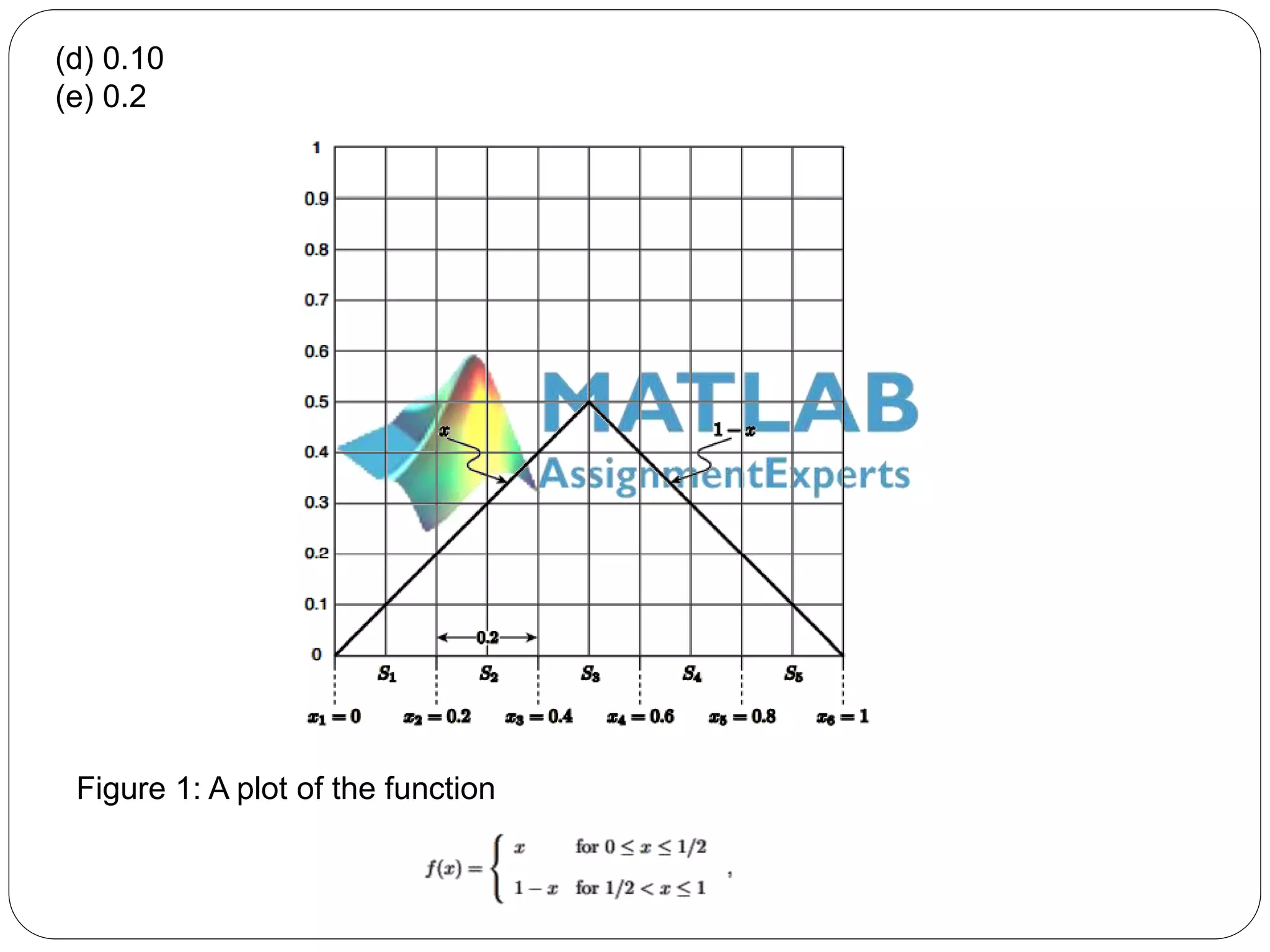
3. We also introduce a set of points xi = i−1 , 1 ≤ i ≤ 6, which define segments Si = [xi,
xi+1], 5 1 ≤ i ≤ 5 (for example, the first segment, S1, is given by 0 ≤ x ≤ 0.20). The
function f(x), points xi, 1 ≤ i ≤ 6, and segments Si, 1 ≤ i ≤ 5, are depicted in Figure
1. In the below we consider two different interpolation procedures, “piecewise-
constant, left endpoint” and “piecewise-linear,” based on the segments Si, 1 ≤ i ≤ 5.
In each case we evaluate the interpolant of f(x) for any given value of x by first
finding the segment which contains x and then within that segment applying the
particular interpolation procedure indicated. Note your interpolants should not
involve evaluations of the function f(x) at points other than the xi, 1 ≤ i ≤ 6, defined
above.
(i) Let (I0f)(x) be the “piecewise-constant, left endpoint” interpolant of f based on
the segments Si, 1 ≤ i ≤ 5. The error in this “piecewise-constant, left, endpoint”
interpolant at x = 0.3, defined as |f(x = 0.3) − (I0f)(x = 0.3)|, is
(a) 0
(b) 0.05
(c) 0.02
(d) 0.1
(e) 0.2
(ii) Let (I1f)(x) be the “piecewise-linear” interpolant of f based on the segments Si, 1
≤ i ≤ 5. The error in this “piecewise-linear” interpolant at x = 0.3, defined as |f(x
= 0.3)−(I1f)(x = 0.3)|, is
(a) 0

4. (d) 0.10
(e) 0.2
Figure 1: A plot of the function

5. as well as the points xi, 1 ≤ i ≤ 6, and associated segments Si, 1 ≤ i ≤ 5. Note the
points xi, 1 ≤ i ≤ 6, are equidistant, and hence the segments Si, 1 ≤ i ≤ 5, are all the
same length 0.2.
Question 3. The function f(x) is defined over the interval 0 ≤ x ≤ 1 by
We also introduce a set of points xi = i−1 , 1 ≤ i ≤ 6, which define segments Si = [xi,
xi+1], 5 1 ≤ i ≤ 5 (for example, the first segment, S1, is given by 0 ≤ x ≤ 0.20). The
function f(x), points xi, 1 ≤ i ≤ 6, and segments Si, 1 ≤ i ≤ 5, are depicted in Figure
1. We further define the definite integral
In the below we shall consider two different numerical approximations to this
integral , “rectangle rule, left” and “trapezoidal rule,” based on the particular
segments Si, 1 ≤ i ≤ 5. Note your numerical approximations should not involve
evaluations of the function f(x) at points other than the xi, 1 ≤ i ≤ 6, defined above.
(i) Let Ih be the “rectangle rule, left” approximation to the integral I. The error in
this 0, left “rectangle rule, left” approximation, defined as |I − I |, is h
(a) 0
(b) 0.01
(c) 0.06

6. (ii) Let I1 be the “trapezoidal rule” approximation to the integral I. The error in this
“trapezoidal h rule” approximation, defined as |I − I1|, is h
(a) 0
(b) 0.01
(c) 0.06
(d) 0.09
(e) 0.2
Question 4. We consider the differentiation of a very smooth function f(x) by finite
differences. 2 (The function is very smooth, but not constant — for example, f(x)
might be x ex.) You are given the values of f(x) at three points x˜1, ˜x2, and x˜3
which are equi-spaced in the sense that x˜2 −x˜1 = h and x˜3 − x˜2 = h; you wish
to approximate the first derivative of f at the particular point x = x˜2, f' (˜x2). The
following finite difference formulas are proposed to approximate f' (˜x2):
(a)
(b)
(c)
(d)

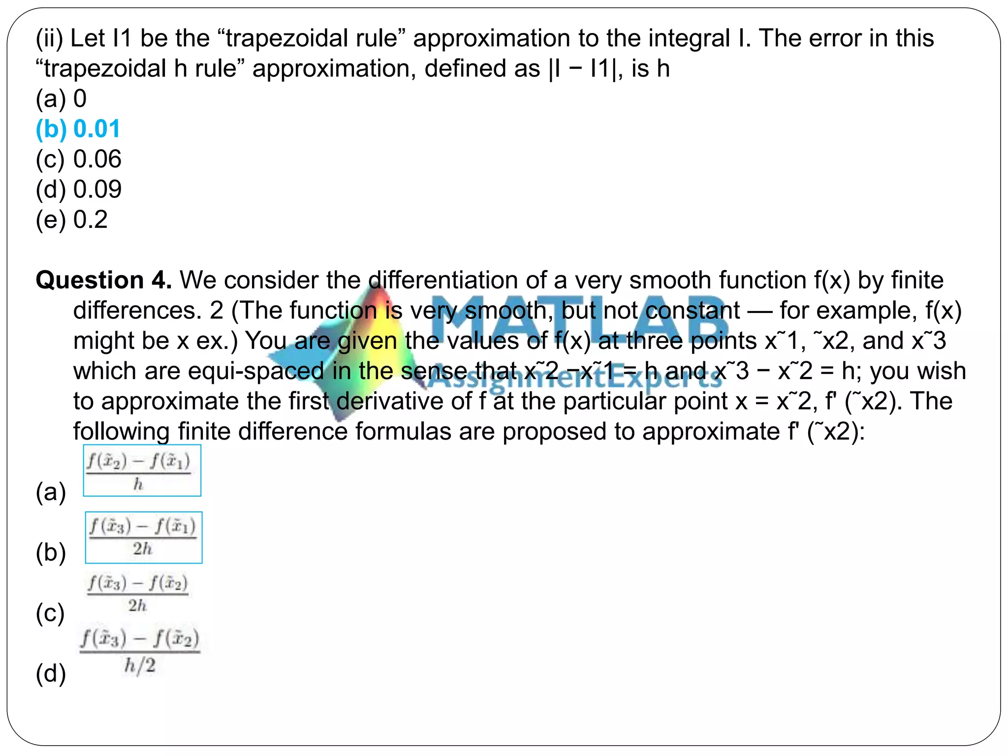
7. (i) Circle all answers which converge to f' (˜x2) as h tends to zero. You will get full
credit for circling all the correct answers and no incorrect answers, proportional
partial credit for circling some of the correct answer(s) and no incorrect
answers, and zero credit if you circle any incorrect answers. (Hint: If the
formula gives the wrong result for a linear function f(x) then certainly the
formula can not converge to the correct result in general.)
(ii) Mark “BEST” next to the answer above which will give the most accurate
approximation to f' (˜x2) (for h sufficiently small).
Question 5. Consider the Matlab script
clear
y = [5,-3,2,7];
val = y(1);
for i = 2:length(y)
% either && or & will work in the statement below
if ( (y(i) <= val) && (y(i) >= 0) )
val = y(i);
end
end
val_save = val

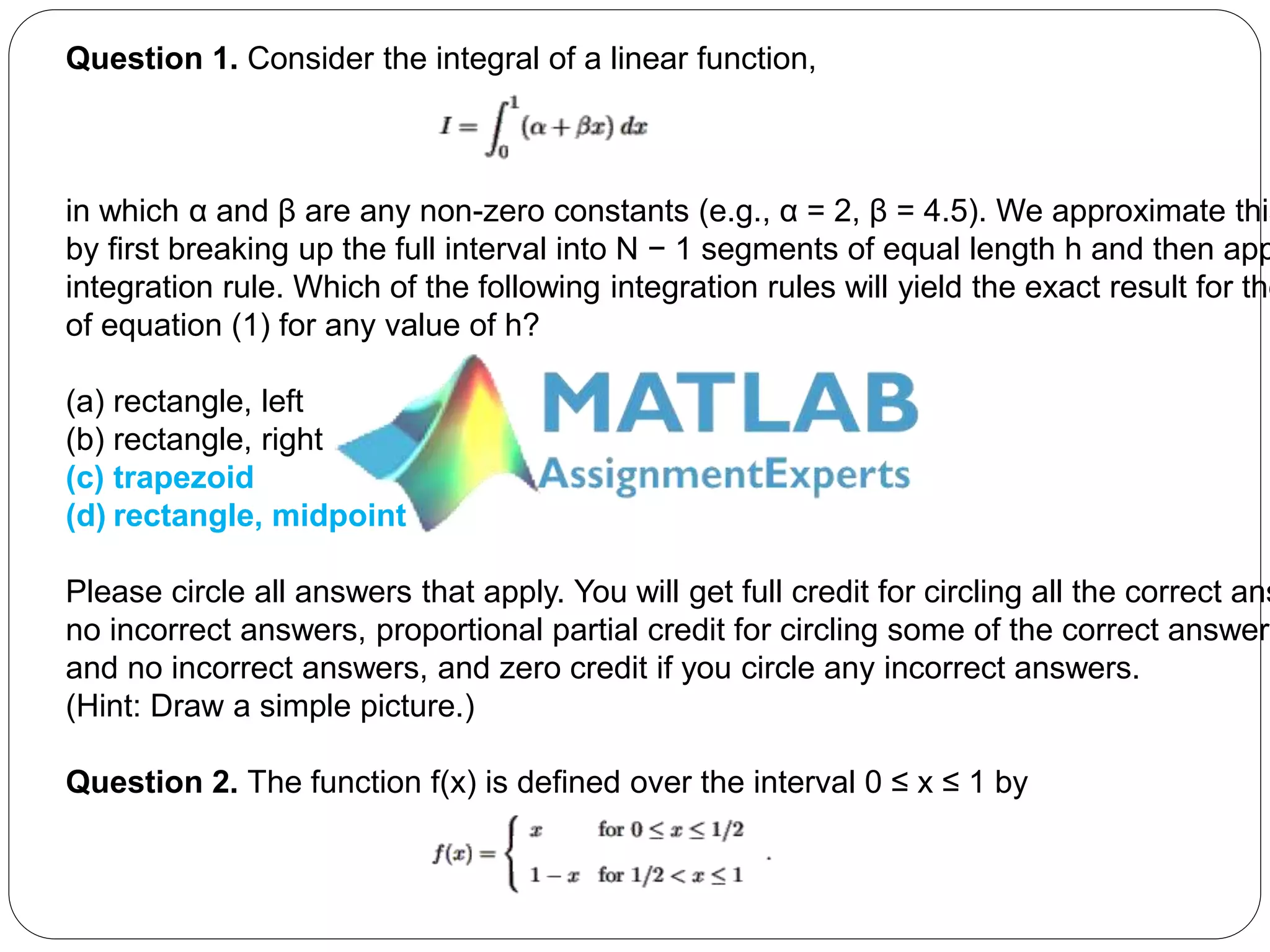
8. (i) The first time through the loop, when i = 2, the expression (y(i) <= val) will
evaluate to
(a) (logical) 0
(b) (logical) 1
(c) 5
(d) -3
where logical here refers to the logical data type or class
(ii) Upon running the script above (to completion) val_save will have the value
(a) 5
(b) -3
(c) 2
(d) 7
Question 6. Consider the Matlab script
clear
x = [1,0,0,2];
y = [0,2,4,5];
z = (x.^2) + y;
ind_vec = find( z > 3 );
r = z(ind_vec);
(i) This script will calculate z to be
(a) [1,2,4,7]

9. (b) [1,2,4,9]
(c) [2,2,4,9]
(d) [1,0,0]
(ii) This script will calculate ind_vec to be
(a) [0,0,1,1]
(b) [0,1,1,0]
(c) [2,3]
(d) [3,4]
(iii) This script will calculate r to be
(a) [4,7]
(b) [4,9]
(c) [3,4]
(d) [25]
Question 7. We wish to approximate the integral
by two different approaches (A and B) in the script
% begin script

10. clear numpts = 21; % number of points in x
h = 1/(numpts-1); % distance between points in x
xpts = h*[0:numpts-1]; % points in x
fval_at_xpts = xpts.*exp(xpts);
weight_vecA = [0,h*ones(1,numpts-1)];
weight_vecB = [0.5*h,h*ones(1,numpts-2),0.5*h];
IA = sum(weight_vecA.*fval_at_xpts);
IB = sum(weight_vecB.*fval_at_xpts);
% end script
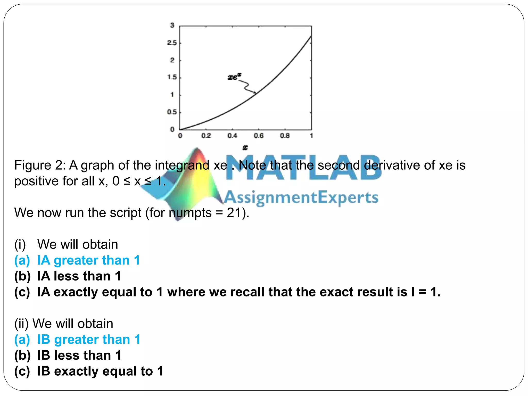
The first approach (A) yields IA; the second approach (B) yields IB. We can readily
derive (by integration by parts) that the exact result is I = 1.
Hint: Run the script “by hand” for numpts = 3 and draw a picture representing the
areas associated with IA and IB. The graph in Figure 2 may prove helpful.

11. Figure 2: A graph of the integrand xe . Note that the second derivative of xe is
positive for all x, 0 ≤ x ≤ 1.
We now run the script (for numpts = 21).
(i) We will obtain
(a) IA greater than 1
(b) IA less than 1
(c) IA exactly equal to 1 where we recall that the exact result is I = 1.
(ii) We will obtain
(a) IB greater than 1
(b) IB less than 1
(c) IB exactly equal to 1

12. (iii) We will find
(a) abs(IA - 1) less than abs(IB - 1)
(b) abs(IA - 1) greater than abs(IB - 1)
(c) abs(IA - 1) equal to abs(IB - 1)
Note that abs is the Matlab built-in absolute value function: abs(z) returns the
absolute value of z. Hence in (iii) we are comparing the absolute value of error
in the two approaches.