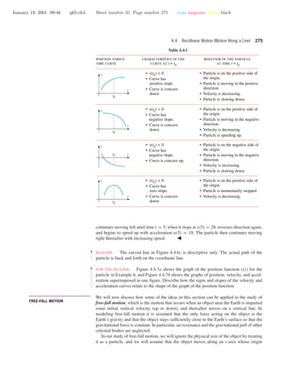
The document discusses analyzing functions using calculus concepts like derivatives. It introduces analyzing functions to determine if they are increasing, decreasing, or constant on intervals based on the sign of the derivative. The sign of the derivative indicates whether the graph of the function has positive, negative, or zero slope at points, relating to whether the function is increasing, decreasing, or constant. It also introduces the concept of concavity, where the derivative indicates whether the curvature of the graph is upward (concave up) or downward (concave down) based on whether tangent lines have increasing or decreasing slopes. Examples are provided to demonstrate these concepts.
![January 19, 2001 09:46 g65-ch4 Sheet number 2 Page number 242 cyan magenta yellow black
242 The Derivative in Graphing and Applications
4.1 ANALYSIS OF FUNCTIONS I: INCREASE, DECREASE,
AND CONCAVITY
Although graphing utilities are useful for determining the general shape of a graph,
many problems require more precision than graphing utilities are capable of produc-
ing. The purpose of this section is to develop mathematical tools that can be used to
determine the exact shape of a graph and the precise locations of its key features.
• • • • • • • • • • • • • • • • • • • • • • • • • • • • • • • • • • • • • •
INCREASING AND DECREASING
FUNCTIONS
Suppose that a function f is differentiable at x0 and that f (x0) > 0. Since the slope of the
graph of f at the point P(x0, f(x0)) is positive, we would expect that a point Q(x, f(x))
on the graph of f that is just to the left of P would be lower than P, and we would expect
that Q would be higher than P if Q is just to the right of P. Analytically, to see why this
is the case, recall that
f (x0) = lim
x →x0
f(x) − f(x0)
x − x0
(Definition 3.2.1 with x1 replaced by x). Since 0 < f (x0), it follows that
0 <
f(x) − f(x0)
x − x0
for values of x very close to (but not equal to) x0. However, for the difference quotient
f(x) − f(x0)
x − x0
to be positive, its numerator f(x) − f(x0) and its denominator x − x0 must have the same
sign. Therefore, for values of x very close to x0, we must have
f(x) − f(x0) < 0 when x − x0 < 0
and
0 < f(x) − f(x0) when 0 < x − x0
Equivalently, f(x) < f(x0) for values of x just to the left of x0, and f(x0) < f(x) for
values of x just to the right of x0. These inequalities confirm our expectation about the
relative positions of P and Q. Similarly, if f (x0) < 0, then f(x) > f(x0) for values of x
just to the left of x0, and f(x0) > f(x) for values of x just to the right of x0. Geometrically,
this means that our point Q would be higher than P if Q is just to the left of P, and that Q
would be lower than P if Q is just to the right of P .
Our next goal is to relate the sign of the derivative of a function f and the relative positions
of points on the graph of f over an entire interval. The terms increasing, decreasing, and
constant are used to describe the behavior of a function over an interval as we travel left to
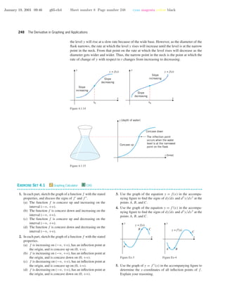
right along its graph. For example, the function graphed in Figure 4.1.1 can be described
as increasing on the interval (−ϱ, 0], decreasing on the interval [0, 2], increasing again on
the interval [2, 4], and constant on the interval [4, +ϱ).
xIncreasing Decreasing Increasing Constant
0 2 4
Figure 4.1.1](https://image.slidesharecdn.com/ch04-150306071940-conversion-gate01/85/Ch04-2-320.jpg)
![January 19, 2001 09:46 g65-ch4 Sheet number 3 Page number 243 cyan magenta yellow black
4.1 Analysis of Functions I: Increase, Decrease, and Concavity 243
The following definition, which is illustrated in Figure 4.1.2, expresses these intuitive
ideas precisely.
4.1.1 DEFINITION. Let f be defined on an interval, and let x1 and x2 denote numbers
in that interval.
(a) f is increasing on the interval if f(x1) < f(x2) whenever x1 < x2.
(b) f is decreasing on the interval if f(x1) > f(x2) whenever x1 < x2.
(c) f is constant on the interval if f(x1) = f(x2) for all x1 and x2.
Increasing Decreasing
f(x1)
f(x2) f(x1)
f(x2)
f(x2)f(x1)
f(x1) > f(x2) if x1 < x2f(x1) < f(x2) if x1 < x2 f(x1) = f(x2) for all x1 and x2
Constant
(a) (b) (c)
x1 x2x1 x2x1 x2
Figure 4.1.2
Figure 4.1.3 suggests that a differentiable function f is increasing on any interval where
its graph has positive slope, is decreasing on any interval where its graph has negative slope,
and is constant on any interval where its graph has zero slope. This intuitive observation
suggests the following important theorem that will be proved in Section 4.8.
Graph has
zero slope.
Graph has
negative slope.
Graph has
positive slope.
x x x
y y y
Figure 4.1.3
4.1.2 THEOREM. Let f be a function that is continuous on a closed interval [a, b]
and differentiable on the open interval (a, b).
(a) If f (x) > 0 for every value of x in (a, b), then f is increasing on [a, b].
(b) If f (x) < 0 for every value of x in (a, b), then f is decreasing on [a, b].
(c) If f (x) = 0 for every value of x in (a, b), then f is constant on [a, b].](https://image.slidesharecdn.com/ch04-150306071940-conversion-gate01/85/Ch04-3-320.jpg)
![January 19, 2001 09:46 g65-ch4 Sheet number 4 Page number 244 cyan magenta yellow black
244 The Derivative in Graphing and Applications
••
•
•
•
•
•
•
•
•
•
•
•
•
•
•
•
•
•
•
•
•
•
•
•
•
•
•
•
•
•
•
•
•
REMARK. Observe that in Theorem 4.1.2 it is only necessary to examine the derivative of
f on the open interval (a, b) to determine whether f is increasing, decreasing, or constant
on the closed interval [a, b]. Moreover, although this theorem was stated for a closed interval
[a, b], it is applicable to any interval I on which f is continuous and inside of which f is
differentiable. For example, if f is continuous on [a, +ϱ) and f (x) > 0 for each x in the
interval (a, +ϱ), then f is increasing on [a, +ϱ); and if f (x) < 0 on (−ϱ, +ϱ), then f is
decreasing on (−ϱ, +ϱ) [the continuity on (−ϱ, +ϱ) follows from the differentiability].
Example 1 Find the intervals on which the following functions are increasing and the
intervals on which they are decreasing.
(a) f(x) = x2
− 4x + 3 (b) f(x) = x3
Solution (a). The graph of f in Figure 4.1.4 suggests that f is decreasing for x ≤ 2 and
increasing for x ≥ 2. To confirm this, we differentiate f to obtain
f (x) = 2x − 4 = 2(x − 2)
It follows that
f (x) < 0 if −ϱ < x < 2
f (x) > 0 if 2 < x < +ϱ
Since f is continuous at x = 2, it follows from Theorem 4.1.2 and the subsequent remark
that
f is decreasing on (−ϱ, 2]
f is increasing on [2, +ϱ)
These conclusions are consistent with the graph of f in Figure 4.1.4.
-1 52
-1
7
f(x) = x2
– 4x + 3
x
y
Figure 4.1.4
-3 3
-4
4
f(x) = x3
x
y
Figure 4.1.5
Solution (b). The graph of f in Figure 4.1.5 suggests that f is increasing over the entire
x-axis. To confirm this, we differentiate f to obtain f (x) = 3x2
. Thus,
f (x) > 0 if −ϱ < x < 0
f (x) > 0 if 0 < x < +ϱ
Since f is continuous at x = 0,
f is increasing on (−ϱ, 0]
f is increasing on [0, +ϱ)
Hence f is increasing over the entire interval (−ϱ, +ϱ), which is consistent with the graph
in Figure 4.1.5 (see Exercise 47).
Example 2
(a) Use the graph of f(x) = 3x4
+ 4x3
− 12x2
+ 2 in Figure 4.1.6 to make a conjecture
about the intervals on which f is increasing or decreasing.
(b) Use Theorem 4.1.2 to determine whether your conjecture is correct.-3 3
-30
20
x
y
f(x) = 3x4
+ 4x3
– 12x2
+ 2
Figure 4.1.6
Solution (a). The graph suggests that f is decreasing if x ≤ −2, increasing if −2 ≤ x ≤ 0,
decreasing if 0 ≤ x ≤ 1, and increasing if x ≥ 1.
Solution (b). Differentiating f we obtain
f (x) = 12x3
+ 12x2
− 24x = 12x(x2
+ x − 2) = 12x(x + 2)(x − 1)
The sign analysis of f in Table 4.1.1 can be obtained using the method of test values
discussed in Appendix A. The conclusions in that table confirm the conjecture in part (a).](https://image.slidesharecdn.com/ch04-150306071940-conversion-gate01/85/Ch04-4-320.jpg)
![January 19, 2001 09:46 g65-ch4 Sheet number 5 Page number 245 cyan magenta yellow black
4.1 Analysis of Functions I: Increase, Decrease, and Concavity 245
Table 4.1.1
interval (12x)(x + 2)(x – 1) conclusion
f is decreasing on (–∞, –2]
f is increasing on [–2, 0]
f is decreasing on [0, 1]
f is increasing on [1, +∞)
(–)
(–)
(+)
(+)
(–)
(+)
(+)
(+)
(–)
(–)
(–)
(+)
f ′(x)
–
+
–
+
x < –2
1 < x
0 < x < 1
–2 < x < 0
• • • • • • • • • • • • • • • • • • • • • • • • • • • • • • • • • • • • • •
CONCAVITY
Although the sign of the derivative of f reveals where the graph of f is increasing or
decreasing, it does not reveal the direction of curvature. For example, on both sides of the
point in Figure 4.1.7 the graph is increasing, but on the left side it has an upward curvature
(“holds water”) and on the right side it has a downward curvature (“spills water”). On
intervals where the graph of f has upward curvature we say that f is concave up, and on
intervals where the graph has downward curvature we say that f is concave down.
Concave
up
“holds
water”
Concave
down
“spills
water”
Figure 4.1.7
For differentiable functions, the direction of curvature can be characterized in terms of
the tangent lines in two ways: As suggested by Figure 4.1.8, the graph of a function f
has upward curvature on intervals where the graph lies above its tangent lines, and it has
downward curvature on intervals where it lies below its tangent lines. Alternatively, the
graph has upward curvature on intervals where the tangent lines have increasing slopes and
downward curvature on intervals where they have decreasing slopes. We will use this latter
characterization as our formal definition.
4.1.3 DEFINITION. If f is differentiable on an open interval I, then f is said to be
concave up on I if f is increasing on I, and f is said to be concave down on I if f is
decreasing on I.
To apply this definition we need some way to determine the intervals on which f is
increasing or decreasing. One way to do this is to apply Theorem 4.1.2 (and the remark
that follows it) to the function f . It follows from that theorem and remark that f will be
increasing where its derivative f is positive and will be decreasing where its derivative f
is negative. This is the idea behind the following theorem.
4.1.4 THEOREM. Let f be twice differentiable on an open interval I.
(a) If f (x) > 0 on I, then f is concave up on I.
(b) If f (x) < 0 on I, then f is concave down on I.
x
y
Concave
down
(spills water)
x
y
Concave
up
(holds water)
Figure 4.1.8
Example 3 Find open intervals on which the following functions are concave up and
open intervals on which they are concave down.
(a) f(x) = x2
− 4x + 3 (b) f(x) = x3
(c) f(x) = x3
− 3x2
+ 1
Solution (a). Calculating the first two derivatives we obtain
f (x) = 2x − 4 and f (x) = 2
Since f (x) > 0 for all x, the function f is concave up on (−ϱ, +ϱ). This is consistent
with Figure 4.1.4.
Solution (b). Calculating the first two derivatives we obtain
f (x) = 3x2
and f (x) = 6x
Since f (x) < 0 if x < 0 and f (x) > 0 if x > 0, the function f is concave down on
(−ϱ, 0) and concave up on (0, +ϱ). This is consistent with Figure 4.1.5.](https://image.slidesharecdn.com/ch04-150306071940-conversion-gate01/85/Ch04-5-320.jpg)
![January 19, 2001 09:46 g65-ch4 Sheet number 7 Page number 247 cyan magenta yellow black
4.1 Analysis of Functions I: Increase, Decrease, and Concavity 247
Table 4.1.2
interval conclusionsign of f′′
3
–1 – √7
x < f is concave up
f is concave down
f is concave up
+
–
+
3
–1 + √7
3
–1 – √7
< x <
3
–1 + √7
< x
1 2 3 4 5 6
-1
1
x
y
f(x) = sin x, 0 ≤ x ≤ o
Figure 4.1.12
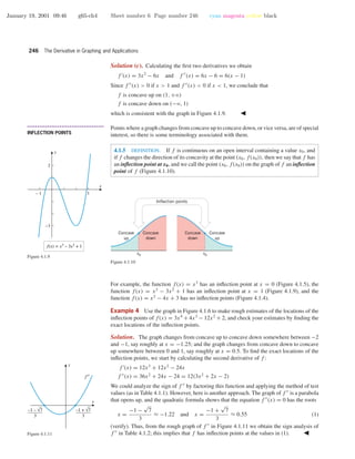
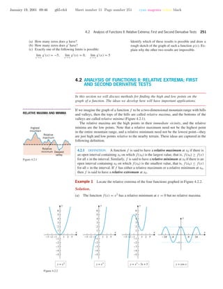
Example 5 Find the inflection points of f(x) = sin x on [0, 2π], and confirm that your
results are consistent with the graph of the function.
Solution. Calculating the first two derivatives of f we obtain
f (x) = cos x, f (x) = − sin x
Thus, f (x) < 0 if 0 < x < π, and f (x) > 0 if π < x < 2π, which implies that the
graph is concave down for 0 < x < π and concave up for π < x < 2π. Thus, there is an
inflection point at x = π ≈ 3.14 (Figure 4.1.12).
••
•
•
•
•
•
•
•
•
•
•
•
•
FOR THE READER. If you have a CAS, devise a method for using it to find exact values
for the inflection points of a function f , and use your method to find the inflection points
of f(x) = x/(x2
+ 1). Verify that your results are consistent with the graph of f .
Intheprecedingexamplestheinflectionpointsoff occurredwheref (x) = 0.However,
inflection points do not always occur where f (x) = 0. Here is a specific example.
Example 6 Find the inflection points, if any, of f(x) = x4
.
Solution. Calculating the first two derivatives of f we obtain
f (x) = 4x3
, f (x) = 12x2
Here f (x) > 0 for x < 0 and for x > 0, which implies that f is concave up for x < 0
and for x > 0 (In fact, f is concave up on (−ϱ, +ϱ.). Thus, there are no inflection points;
and in particular, there is no inflection point at x = 0, even though f (0) = 0 (Figure
4.1.13).
-2 2
4
f(x) = x4
x
y
Figure 4.1.13
••
•
•
•
•
•
•
FOR THE READER. An inflection point may occur at a point of nondifferentiability. Verify
that this is the case for x1/3
at x = 0.
• • • • • • • • • • • • • • • • • • • • • • • • • • • • • • • • • • • • • •
INFLECTION POINTS IN
APPLICATIONS
Up to now we have viewed the inflection points of a curve y = f(x) as those points where the
curve changes the direction of its concavity. However, inflection points also mark the points
on the curve where the slopes of the tangent lines change from increasing to decreasing, or
vice versa (Figure 4.1.14); stated another way:
Inflection points mark the places on the curve y = f(x) where the rate of change of y
with respect to x changes from increasing to decreasing, or vice versa.
Note that we are dealing with a rather subtle concept here—a change of a rate of change.
However, the following physical example should help to clarify the idea: Suppose that water
is added to the flask in Figure 4.1.15 in such a way that the volume increases at a constant
rate, and let us examine the rate at which the water level y rises with the time t. Initially,](https://image.slidesharecdn.com/ch04-150306071940-conversion-gate01/85/Ch04-7-320.jpg)
![January 19, 2001 09:46 g65-ch4 Sheet number 9 Page number 249 cyan magenta yellow black
4.1 Analysis of Functions I: Increase, Decrease, and Concavity 249
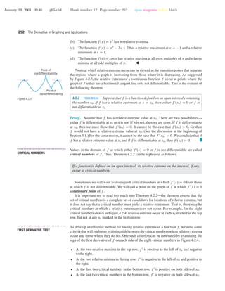
6. Use the graph of y = f (x) in the accompanying figure to
replace the question mark with <, =, or >, as appropriate.
Explain your reasoning.
(a) f(0) ? f(1) (b) f(1) ? f(2) (c) f (0) ? 0
(d) f (1) ? 0 (e) f (0) ? 0 (f) f (2) ? 0
-2 3
x
y
y = f′′(x)
Figure Ex-5
21
x
y
y = f′(x)
Figure Ex-6
7. In each part, use the graph of y = f(x) in the accompanying
figure to find the requested information.
(a) Find the intervals on which f is increasing.
(b) Find the intervals on which f is decreasing.
(c) Find the open intervals on which f is concave up.
(d) Find the open intervals on which f is concave down.
(e) Find all values of x at which f has an inflection point.
2
3 4
5 6 71
x
y
y = f(x)
Figure Ex-7
8. Use the graph in Exercise 7 to make a table that shows the
signs of f and f over the intervals (1, 2), (2, 3), (3, 4),
(4, 5), (5, 6), and (6, 7).
In Exercises 9 and 10, a sign chart is presented for the first
and second derivatives of a function f . Assuming that f is
continuous everywhere, find: (a) the intervals on which f is
increasing, (b) the intervals on which f is decreasing, (c) the
open intervals on which f is concave up, (d) the open inter-
vals on which f is concave down, and (e) the x-coordinates
of all inflection points.
9.
interval sign of f ″(x)sign of f ′(x)
–
+
+
–
–
+
+
–
–
+
x < 1
3 < x < 4
2 < x < 3
4 < x
1 < x < 2
10.
interval sign of f ″(x)sign of f ′(x)
+
+
+
+
–
+
x < 1
3 < x
1 < x < 3
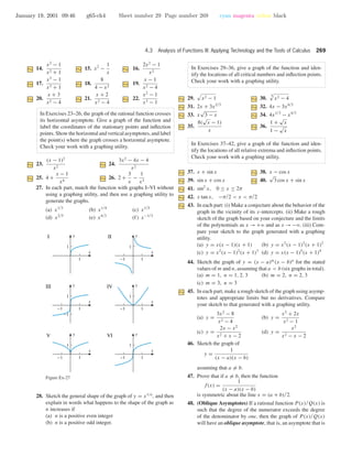
In Exercises 11–22, find: (a) the intervals on which f is in-
creasing, (b) the intervals on which f is decreasing, (c) the
open intervals on which f is concave up, (d) the open inter-
vals on which f is concave down, and (e) the x-coordinates
of all inflection points.
11. f(x) = x2
− 5x + 6 12. f(x) = 4 − 3x − x2
13. f(x) = (x + 2)3
14. f(x) = 5 + 12x − x3
15. f(x) = 3x4
− 4x3
16. f(x) = x4
− 8x2
+ 16
17. f(x) =
x2
x2 + 2
18. f(x) =
x
x2 + 2
19. f(x) =
3√
x + 2 20. f(x) = x2/3
21. f(x) = x1/3
(x + 4) 22. f(x) = x4/3
− x1/3
In Exercises 23–28, analyze the trigonometric function f
over the specified interval, stating where f is increasing, de-
creasing, concave up, and concave down, and stating the x-
coordinates of all inflection points. Confirm that your results
are consistent with the graph of f generated with a graphing
utility.
23. f(x) = cos x; [0, 2π]
24. f(x) = sin2
2x; [0, π]
25. f(x) = tan x; (−π/2, π/2)
26. f(x) = 2x + cot x; (0, π)
27. f(x) = sin x cos x; [0, π]
28. f(x) = cos2
x − 2 sin x; [0, 2π]
29. In each part sketch a continuous curve y = f(x) with the
stated properties.
(a) f(2) = 4, f (2) = 0, f (x) > 0 for all x
(b) f(2) = 4, f (2) = 0, f (x) < 0 for x < 2, f (x) > 0
for x > 2
(c) f(2) = 4, f (x) < 0forx = 2and lim
x →2+
f (x) = +ϱ,
lim
x →2−
f (x) = −ϱ
30. In each part sketch a continuous curve y = f(x) with the
stated properties.
(a) f(2) = 4, f (2) = 0, f (x) < 0 for all x
(b) f(2) = 4, f (2) = 0, f (x) > 0 for x < 2, f (x) < 0
for x > 2
(c) f(2) = 4, f (x) > 0forx = 2and lim
x →2+
f (x) = −ϱ,
lim
x →2−
f (x) = +ϱ
31. In each part, assume that a is a constant and find the inflec-
tion points, if any.
(a) f(x) = (x − a)3
(b) f(x) = (x − a)4](https://image.slidesharecdn.com/ch04-150306071940-conversion-gate01/85/Ch04-9-320.jpg)
![January 19, 2001 09:46 g65-ch4 Sheet number 10 Page number 250 cyan magenta yellow black
250 The Derivative in Graphing and Applications
32. Given that a is a constant and n is a positive integer, what
can you say about the existence of inflection points of the
function f(x) = (x − a)n
? Justify your answer.
If f is increasing on an interval [0, b), then it follows from
Definition 4.1.1 that f(0) < f(x) for each x in the interval.
Use this result in Exercises 33–36.
33. Show that 3
√
1 + x < 1 + 1
3
x if x > 0, and confirm the in-
equality with a graphing utility. [Hint: Show that the func-
tion f(x) = 1 + 1
3
x − 3
√
1 + x is increasing on [0, +ϱ).]
34. Show that x < tan x if 0 < x < π/2, and confirm the in-
equality with a graphing utility. [Hint: Show that the func-
tion f(x) = tan x − x is increasing on [0, π/2).]
35. Use a graphing utility to make a conjecture about the relative
sizes of x and sin x for x ≥ 0, and prove your conjecture.
36. Use a graphing utility to make a conjecture about the rela-
tive sizes of 1 − x2/2 and cos x for x ≥ 0, and prove your
conjecture. [Hint: Use the result of Exercise 35.]
In Exercises 37 and 38, use a graphing utility to generate the
graphs of f and f over the stated interval; then use those
graphs to estimate the x-coordinates of the inflection points
of f , the intervals on which f is concave up or down, and
the intervals on which f is increasing or decreasing. Check
your estimates by graphing f .
37. f(x) = x4
− 24x2
+ 12x, −5 ≤ x ≤ 5
38. f(x) =
1
1 + x2
, −5 ≤ x ≤ 5
In Exercises 39 and 40, use a CAS to find f and to approxi-
mate the x-coordinates of the inflection points to six decimal
places. Confirm that your answer is consistent with the graph
of f .
C 39. f(x) =
10x − 3
3x2 − 5x + 8
C 40. f(x) =
x3
− 8x + 7
x2 + 1
41. Use Definition 4.1.1 to prove that f(x) = x2
is increasing
on [0, +ϱ).
42. Use Definition 4.1.1 to prove that f(x) = 1/x is decreasing
on (0, +ϱ).
43. In each part, determine whether the statement is true or false.
If it is false, find functions for which the statement fails to
hold.
(a) If f and g are increasing on an interval, then so is f +g.
(b) If f and g are increasing on an interval, then so is f ·g.
44. In each part, find functions f and g that are increasing on
(−ϱ, +ϱ) and for which f − g has the stated property.
(a) f − g is decreasing on (−ϱ, +ϱ).
(b) f − g is constant on (−ϱ, +ϱ).
(c) f − g is increasing on (−ϱ, +ϱ).
45. (a) Prove that a general cubic polynomial
f(x) = ax3
+ bx2
+ cx + d (a = 0)
has exactly one inflection point.
(b) Prove that if a cubic polynomial has three x-intercepts,
then the inflection point occurs at the average value of
the intercepts.
(c) Use the result in part (b) to find the inflection point of the
cubic polynomial f(x) = x3
−3x2
+2x, and check your
result by using f to determine where f is concave up
and concave down.
46. From Exercise 45, the polynomial f(x) = x3
+ bx2
+ 1
has one inflection point. Use a graphing utility to reach a
conclusion about the effect of the constant b on the location
of the inflection point. Use f to explain what you have
observed graphically.
47. Use Definition 4.1.1 to prove:
(a) If f is increasing on the intervals (a, c] and [c, b), then
f is increasing on (a, b).
(b) If f is decreasing on the intervals (a, c] and [c, b), then
f is decreasing on (a, b).
48. Use part (a) of Exercise 47 to show that f(x) = x + sin x
is increasing on the interval (−ϱ, +ϱ).
49. Use part (b) of Exercise 47 to show that f(x) = cos x − x
is decreasing on the interval (−ϱ, +ϱ).
50. Let y = 1/(1 + x2
). Find the values of x for which y is
increasing most rapidly or decreasing most rapidly.
In Exercises 51 and 52, suppose that water is flowing at a
constant rate into the container shown. Make a rough sketch
of the graph of the water level y versus the time t. Make sure
that your sketch conveys where the graph is concave up and
concave down, and label the y-coordinates of the inflection
points.
51. y
1
0
2
52. y
1
0
2
3
4
53. Suppose that g(x) is a function that is defined and differen-
tiable for all real numbers x and that g(x) has the following
properties:
(i) g(0) = 2 and g (0) = −2
3
.
(ii) g(4) = 3 and g (4) = 3.
(iii) g(x) is concave up for x < 4 and concave down for
x > 4.
(iv) g(x) ≥ −10 for all x.](https://image.slidesharecdn.com/ch04-150306071940-conversion-gate01/85/Ch04-10-320.jpg)
![January 19, 2001 09:46 g65-ch4 Sheet number 13 Page number 253 cyan magenta yellow black
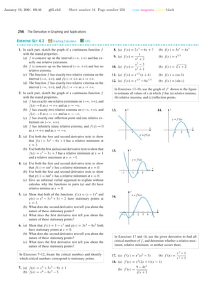
4.2 Analysis of Functions II: Relative Extrema; First and Second Derivative Tests 253
x
y
x0
x
y
x0
x
y
x0
x
y
x0
x
y
x0
x
y
x0
x
y
x0
x
y
x0
Figure 4.2.4
These observations suggest that a function f will have relative extrema at those critical
numbers, and only those critical numbers, where f changes sign. Moreover, if the sign
changes from positive to negative, then a relative maximum occurs; and if the sign changes
fromnegativetopositive,thenarelativeminimumoccurs.Thisisthecontentofthefollowing
theorem.
4.2.3 THEOREM (First Derivative Test). Suppose f is continuous at a critical number x0.
(a) If f (x) > 0 on an open interval extending left from x0 and f (x) < 0 on an open
interval extending right from x0, then f has a relative maximum at x0.
(b) If f (x) < 0 on an open interval extending left from x0 and f (x) > 0 on an open
interval extending right from x0, then f has a relative minimum at x0.
(c) If f (x) has the same sign [either f (x) > 0 or f (x) < 0] on an open interval
extending left from x0 and on an open interval extending right from x0, then f does
not have a relative extremum at x0.
We will prove part (a) and leave parts (b) and (c) as exercises.
Proof. We are assuming that f (x) > 0 on the interval (a, x0) and that f (x) < 0 on the
interval (x0, b), and we want to show that
f(x0) ≥ f(x)
for all x in the interval (a, b). However, the two hypotheses, together with Theorem 4.1.2
(and its following remark), imply that f is increasing on the interval (a, x0] and decreasing
on the interval [x0, b). Thus, f(x0) ≥ f(x) for all x in (a, b) with equality only at x0.
Example 2
(a) Locate the relative maxima and minima of f(x) = 3x5/3
− 15x2/3
.
(b) Confirm that the results in part (a) agree with the graph of f .
Solution (a). The function f is defined and continuous for all real values of x, and its
derivative is
f (x) = 5x2/3
− 10x−1/3
= 5x−1/3
(x − 2) =
5(x − 2)
x1/3
Since f (x) does not exist if x = 0, and since f (x) = 0 if x = 2, there are critical numbers at](https://image.slidesharecdn.com/ch04-150306071940-conversion-gate01/85/Ch04-13-320.jpg)
![January 19, 2001 09:46 g65-ch4 Sheet number 14 Page number 254 cyan magenta yellow black
254 The Derivative in Graphing and Applications
x = 0 and x = 2. To apply the first derivative test, we examine the sign of f (x) on intervals
extending to the left and right of the critical numbers (Figure 4.2.5). Since the sign of the
derivative changes from positive to negative at x = 0, there is a relative maximum there,
and since it changes from negative to positive at x = 2, there is a relative minimum there.
0 2
+ + + 0 – – – – – 0 + + + +
Sign of f ′(x) = 5x–1/3
(x – 2)
x
Figure 4.2.5
Solution(b). Theresultinpart(a)agreeswiththegraphoff showninFigure4.2.6.
[–2, 10] × [–15, 20]
xScl = 2, yScl = 5
f(x) = 3x5/3
– 15x2/3
Figure 4.2.6
••
•
•
•
•
•
•
•
•
•
•
•
•
•
•
•
•
•
•
•
•
•
•
•
•
•
•
•
•
•
•
•
•
FOR THE READER. As discussed in the subsection of Section 1.3 entitled Errors of Omis-
sion, many graphing utilities omit portions of the graphs of functions with fractional expo-
nents and must be “tricked” into producing complete graphs; and indeed, for the function in
the last example both a calculator and a CAS failed to produce the portion of the graph over
the negative x-axis. To generate the graph in Figure 4.2.6, apply the techniques discussed
in Exercise 29 of Section 1.3 to each term in the formula for f . Use a graphing utility to
generate this graph.
Example 3 Locate the relative extrema of f(x) = x3
− 3x2
+ 3x − 1, if any.
Solution. Since f is differentiable everywhere, the only possible critical numbers corre-
spond to stationary points. Differentiating f yields
f (x) = 3x2
− 6x + 3 = 3(x − 1)2
Solving f (x) = 0 yields only x = 1. However, 3(x − 1)2
≥ 0 for all x, so f (x) does not
change sign at x = 1; consequently, f does not have a relative extremum at x = 1. Thus,
f has no relative extrema (Figure 4.2.7).
-1 1 2 3
-2
-1
1
2
x
y
f(x) = x3
– 3x2
+ 3x – 1
Figure 4.2.7
••
•
•
•
•
•
•
FOR THE READER. How many relative extrema can a polynomial of degree n have? Ex-
plain your reasoning.
• • • • • • • • • • • • • • • • • • • • • • • • • • • • • • • • • • • • • •
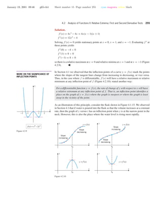
SECOND DERIVATIVE TEST
There is another test for relative extrema that is often easier to apply than the first derivative
test. It is based on the geometric observation that a function f has a relative maximum at a
stationary point if the graph of f is concave down on an open interval containing the point,
and it has a relative minimum if it is concave up (Figure 4.2.8).
f′′ < 0
Concave down
f ′′ > 0
Concave up
Relative
maximum
Relative
minimum
Figure 4.2.8
4.2.4 THEOREM (Second Derivative Test). Suppose that f is twice differentiable at x0.
(a) If f (x0) = 0 and f (x0) > 0, then f has a relative minimum at x0.
(b) If f (x0) = 0 and f (x0) < 0, then f has a relative maximum at x0.
(c) If f (x0) = 0 and f (x0) = 0, then the test is inconclusive; that is, f may have a
relative maximum, a relative minimum, or neither at x0.
We will prove parts (a) and (c) and leave part (b) as an exercise.
Proof (a). We are assuming that f (x0) = 0 and f (x0) > 0, and we want to show that
f has a relative minimum at x0. It follows from our discussion at the beginning of Section
4.1 (with the function f replaced by f ) that if f (x0) > 0, then f (x) < f (x0) = 0 for x
just to the left of x0, and f (x) > f (x0) = 0 for x just to the right of x0. But then f has a
relative minimum at x0 by the first derivative test.
Proof (b). Consider the functions f(x) = x3
, f(x) = x4
, and f(x) = −x4
. It is easy to
check that in all three cases f (0) = 0 and f (0) = 0; but from Figure 1.6.4, f(x) = x4
has a relative minimum at x = 0, f(x) = −x4
has a relative maximum at x = 0 (why?),
and f(x) = x3
has neither a relative maximum nor a relative minimum at x = 0.
Example 4 Locate the relative maxima and minima of f(x) = x4
− 2x2
, and confirm
that your results are consistent with the graph of f .](https://image.slidesharecdn.com/ch04-150306071940-conversion-gate01/85/Ch04-14-320.jpg)
![January 19, 2001 09:46 g65-ch4 Sheet number 20 Page number 260 cyan magenta yellow black
260 The Derivative in Graphing and Applications
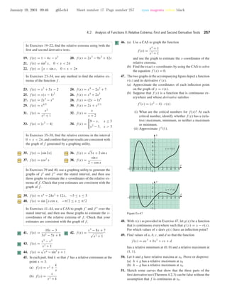
Example 1 Figure 4.3.2 shows the graph of
y = x3
− x2
− 2x
produced on a graphing calculator. Confirm that the graph is not missing any significant
features.
[–2, 3] × [–3, 2]
xScl = 1, yScl = 1
y = x3
– x2
– 2x
Figure 4.3.2
Solution. We can be confident that the graph exhibits all the significant features of the
polynomial because the polynomial has degree 3, and three roots, two relative extrema, and
one inflection point are accounted for. Moreover, the graph indicates the correct behavior
as x →+ϱ and as x →−ϱ, since
lim
x →+ϱ
(x3
− x2
− 2x) = lim
x →+ϱ
x3
= +ϱ
lim
x →−ϱ
(x3
− x2
− 2x) = lim
x →−ϱ
x3
= −ϱ
• • • • • • • • • • • • • • • • • • • • • • • • • • • • • • • • • • • • • •
GEOMETRIC IMPLICATIONS OF
MULTIPLICITY
A root x = r of a polynomial p(x) has multiplicity m if (x−r)m
divides p(x) but (x−r)m+1
does not. A root of multiplicity 1 is called a simple root. There is a close relationship between
the multiplicity of a root of a polynomial and the behavior of the graph in the vicinity of
the root. This relationship, stated below, is illustrated in Figure 4.3.3.
Roots of even multiplicity Roots of odd multiplicity (>1) Simple roots
Figure 4.3.3
4.3.1 THE GEOMETRIC IMPLICATIONS OF MULTIPLICITY. Suppose that p(x) is a
polynomial with a root of multiplicity m at x = r.
(a) If m is even, then the graph of y = p(x) is tangent to the x-axis at x = r, does not
cross the x-axis there and does not have an inflection point there.
(b) If m is odd and greater than 1, then the graph is tangent to the x-axis at x = r,
crosses the x-axis there, and also has an inflection point there.
(c) If m = 1 (so that the root is simple), then the graph is not tangent to the x-axis at
x = r, crosses the x-axis there, and may or may not have an inflection point there.
-3 -2 -1 1 2 3
-10
-5
5
10
x
y
y = x3
(3x – 4)(x + 2)2
Figure 4.3.4
Example 2 Make a conjecture about the behavior of the graph of
y = x3
(3x − 4)(x + 2)2
in the vicinity of its x-intercepts, and test your conjecture by generating the graph.
Solution. The x-intercepts occur at x = 0, x = 4
3
, and x = −2. The root x = 0 has
multiplicity 3, which is odd, so at that point the graph should be tangent to the x-axis, cross
the x-axis, and have an inflection point there. The root x = −2 has multiplicity 2, which
is even, so the graph should be tangent to but not cross the x-axis there. The root x = 4
3
is
simple, so at that point the curve should cross the x-axis without being tangent to it. All of
this is consistent with the graph in Figure 4.3.4.](https://image.slidesharecdn.com/ch04-150306071940-conversion-gate01/85/Ch04-20-320.jpg)
![January 19, 2001 09:46 g65-ch4 Sheet number 21 Page number 261 cyan magenta yellow black
4.3 Analysis of Functions III: Applying Technology and the Tools of Calculus 261
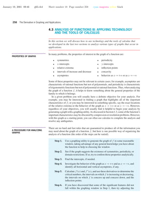
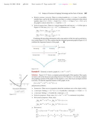
Example 3 Generate or sketch a graph of the equation
y = x3
− 3x + 2 = (x + 2)(x − 1)2
and identify the exact locations of the intercepts, relative extrema, and inflection points.
Solution. Figure 4.3.5 shows a graph of the given equation produced with a graphing
utility. Since the polynomial has degree 3, all roots, relative extrema, and inflection points
are accounted for in the graph: there are three roots (a simple negative root and a positive
root of multiplicity 2), and there are two relative extrema and one inflection point. The
following analysis will identify the exact locations of the intercepts, relative extrema, and
inflection points.
[–10, 10] × [–10, 10]
xScl = 1, yScl = 1
y = x3
– 3x + 2
Figure 4.3.5
• x-intercepts: Setting y = 0 yields roots at x = −2 and at x = 1.
• y-intercept: Setting x = 0 yields y = 2.
• Behavior as x →+ϱ and as x →−ϱ: The graph in Figure 4.3.5 suggests that the graph
increases without bound as x →+ϱ and decreases without bound as x →−ϱ. This is
confirmed by the limits
lim
x →+ϱ
(x3
− 3x + 2) = lim
x →+ϱ
x3
= +ϱ
lim
x →−ϱ
(x3
− 3x + 2) = lim
x →−ϱ
x3
= −ϱ
• Derivatives:
dy
dx
= 3x2
− 3 = 3(x − 1)(x + 1)
d2
y
dx2
= 6x
• Intervals of increase and decrease; relative extrema; concavity: Figure 4.3.6 shows the
sign pattern of the first and second derivatives and what they imply about the graph
shape.
Figure 4.3.7 shows the graph labeled with the coordinates of the intercepts, relative
extrema, and inflection point.
0
–1
0–––––––––––– + + + + + + + + + + + +
Concave down Inflection Concave up
1
0+++++ 0–––––––––––––– + + + + +
Increasing Sta StaDecreasing Increasing
x
dy/dx = 3(x – 1)(x + 1)
y
x
d2
y/dx2
= 6x
y
Rough sketch of
y = x3
– 3x + 2
Figure 4.3.6
-2 -1 1 2
x
y
(–1, 4)
(1, 0)
(0, 2)
(–2, 0)
y = x3
– 3x + 2
Figure 4.3.7
• • • • • • • • • • • • • • • • • • • • • • • • • • • • • • • • • • • • • •
GRAPHING RATIONAL FUNCTIONS
Rational functions (ratios of polynomials) are more complicated to graph than polynomials
because they may have discontinuities and asymptotes.](https://image.slidesharecdn.com/ch04-150306071940-conversion-gate01/85/Ch04-21-320.jpg)
![January 19, 2001 09:46 g65-ch4 Sheet number 22 Page number 262 cyan magenta yellow black
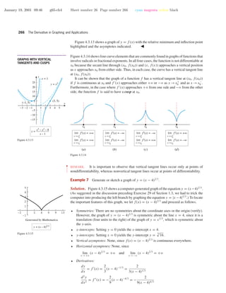
262 The Derivative in Graphing and Applications
Example 4 Generate or sketch a graph of the equation
y =
2x2
− 8
x2 − 16
and identify the exact location of the intercepts, relative extrema, inflection points, and
asymptotes.
[–10, 10] × [–10, 10]
xScl = 1, yScl = 1
y = 2x2
– 8
x2
– 16
Figure 4.3.8
Solution. Figure 4.3.8 shows a calculator-generated graph of the equation in the window
[−10, 10] × [−10, 10]. The figure suggests that the graph is symmetric about the y-axis
and has two vertical asymptotes and a horizontal asymptote. The figure also suggests that
there is a relative maximum at x = 0 and two x-intercepts. There do not seem to be any
inflection points. The following analysis will identify the exact location of the key features
of the graph.
• Symmetries: Replacing x by −x does not change the equation, so the graph is symmetric
about the y-axis.
• x-intercepts: Setting y = 0 yields the x-intercepts x = −2 and x = 2.
• y-intercept: Setting x = 0 yields the y-intercept y = 1
2
.
• Vertical asymptotes: Setting x2
−16 = 0 yields the solutions x = −4 and x = 4. Since
neither solution is a root of 2x2
− 8, the graph has vertical asymptotes at x = −4 and
x = 4.
• Horizontal asymptotes: The limits
lim
x →+ϱ
2x2
− 8
x2 − 16
= lim
x →+ϱ
2 − (8/x2
)
1 − (16/x2)
= 2
lim
x →−ϱ
2x2
− 8
x2 − 16
= lim
x →−ϱ
2 − (8/x2
)
1 − (16/x2)
= 2
yield the horizontal asymptote y = 2.
The set of values where x-intercepts or vertical asymptotes occur is {−4, −2, 2, 4}. These
values divide the x-axis into the open intervals
(−ϱ, −4), (−4, −2), (−2, 2), (2, 4), (4, +ϱ)
Over each of these intervals, y cannot change sign (why?). We can find the sign of y on
each interval by choosing an arbitrary test value in the interval and evaluating y = f(x) at
the test value (Table 4.3.1).
Table 4.3.1
(–∞, –4)
(–4, –2)
(–2, 2)
(2, 4)
(4, +∞)
x = –5
x = –3
x = 0
x = 3
x = 5
y = 14/3
y = –10/7
y = 1/2
y = –10/7
y = 14/3
+
–
+
–
+
interval
test
value sign of y
y = 2x2
– 8
x2
– 16
The information in Table 4.3.1 is consistent with Figure 4.3.8, so we can be certain
that the calculator graph has not missed any sign changes. The next step is to use the first](https://image.slidesharecdn.com/ch04-150306071940-conversion-gate01/85/Ch04-22-320.jpg)
![January 19, 2001 09:46 g65-ch4 Sheet number 23 Page number 263 cyan magenta yellow black
4.3 Analysis of Functions III: Applying Technology and the Tools of Calculus 263
and second derivatives to determine whether the calculator graph has missed any relative
extrema or changes in concavity.
• Derivatives:
dy
dx
=
(x2
− 16)(4x) − (2x2
− 8)(2x)
x2 − 16
2
= −
48x
x2 − 16
2
d2
y
dx2
=
48(16 + 3x2
)
x2 − 16
3
(verify)
• Intervals of increase and decrease; relative extrema: A sign analysis of dy/dx yields
0 4–4
0 ∞∞ – –––– – ––––++++++++++
UndefIncr Incr Sta Decr DecrUndef
x
Sign of dy/dx
y
Thus, the graph is increasing on the intervals (−ϱ, −4) and (−4, 0]; and it is decreasing
on the intervals [0, 4) and (4, +ϱ). There is a relative maximum at x = 0.
• Concavity: A sign analysis of d2
y/dx2
yields
4–4
∞∞ – ––––– ––––+++++ +++++
Concave
up
Concave
down
Concave
up
x
Sign of d2
y/dx2
y
There are changes in concavity at the vertical asymptotes, x = −4 and x = 4, but there
are no inflection points.
This analysis confirms that our calculator-generated graph exhibited all important fea-
tures of the rational function. Figure 4.3.9 shows a graph of the equation with the asymptotes,
intercepts, and relative maximum identified.
-8 -4 4 8
-8
-4
4
8
x
y
y = 2x2
– 8
x2
– 16
Figure 4.3.9
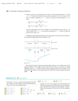
Example 5 Generate or sketch a graph of
y =
x2
− 1
x3
and identify the exact locations of all asymptotes, intercepts, relative extrema, and inflection
points.
Solution. Figure 4.3.10a shows a calculator-generated graph of the given equation in
the window [−10, 10] × [−10, 10], and Figure 4.3.10b shows a second version of the
graph that gives more detail in the vicinity of the x-axis. These figures suggest that the
graph is symmetric about the origin. They also suggest that there are two relative extrema,
two inflection points, two x-intercepts, a vertical asymptote at x = 0, and a horizontal
asymptote at y = 0. The following analysis will identify the exact locations of all the key
features and will determine whether the calculator-generated graphs in Figure 4.3.10 have
missed any of these features.
[–10, 10] × [–10, 10]
xScl = 1, yScl = 1
(a)
[–4, 4] × [–2, 2]
xScl = 1, yScl = 1
(b)
y = x2
– 1
x3
Figure 4.3.10
• Symmetries: Replacing x by −x and y by −y yields an equation that simplifies back to
the original equation, so the graph is symmetric about the origin.
• x-intercepts: Setting y = 0 yields the x-intercepts x = −1 and x = 1.
• y-intercept: Setting x = 0 leads to a division by zero, so that there is no y-intercept.
• Vertical asymptotes: Setting x3
= 0 yields the solution x = 0. This is not a root of
x2
− 1, so x = 0 is a vertical asymptote.](https://image.slidesharecdn.com/ch04-150306071940-conversion-gate01/85/Ch04-23-320.jpg)
![January 19, 2001 09:46 g65-ch4 Sheet number 24 Page number 264 cyan magenta yellow black
264 The Derivative in Graphing and Applications
• Horizontal asymptotes: The limits
lim
x →+ϱ
x2
− 1
x3
= lim
x →+ϱ
1
x
− 1
x3
1
= lim
x →+ϱ
1
x
= 0
lim
x →−ϱ
x2
− 1
x3
= lim
x →−ϱ
1
x
− 1
x3
1
= lim
x →−ϱ
1
x
= 0
yield the horizontal asymptote y = 0.
• Derivatives:
dy
dx
=
x3
(2x) − (x2
− 1)(3x2
)
x3 2
=
3 − x2
x4
d2
y
dx2
=
x4
(−2x) − (3 − x2
)(4x3
)
x4 2
=
2(x2
− 6)
x5
• Intervals of increase and decrease; relative extrema:
0
00 ∞ + ++++ – ––––+++++–––––
StaDecr Incr Undef Incr DecrSta
x
Sign of dy/dx
y
–√3 √3
This analysis reveals a relative minimum at x = −
√
3 and a relative maximum at
x =
√
3.
• Concavity:
0
∞ – – ––––+ + ++++–––– ++++00
Concave
up
Concave
down
Concave
down
Concave
up
InflInfl Undef
x
Sign of d2
y/dx2
y
–√6 √6
This analysis reveals that changes in concavity occur at the vertical asymptote x = 0
and at the inflection points at x = −
√
6 and at x =
√
6.
Figure 4.3.11 shows a table of coordinate values at the relative extrema and inflec-
tion points together with a graph of the equation on which we have emphasized these
points.
-3 -2 -1 1 2 3
-2
-1
1
2
x
y
–√6 ≈ –2.45
–√3 ≈ –1.73
√3 ≈ 1.73
√6 ≈ 2.45
– ≈ –0.38
≈ 0.38
≈ 0.34
5√6
36
– ≈ –0.34
2√3
9
2√3
9
5√6
36
x y = x2
– 1
x3
y = x2
– 1
x3
Figure 4.3.11
Suppose that the numerator polynomial of a rational function f(x) has degree greater
than the degree of the denominator polynomial d(x). Then by division we can write
f(x) = q(x) +
r(x)
d(x)
where q(x) and r(x) are polynomials and the degree of r(x) is less than that of d(x). In
this case, f(x) will be asymptotic to the quotient polynomial q(x); that is,
lim
x →−ϱ
[f(x) − q(x)] = 0 and lim
x →+ϱ
[f(x) − q(x)] = 0
(see the end of Exercise Set 2.3). Exercises 48–54 at the end of this section deal with the
instance of an oblique asymptote, where the numerator has degree one more than the degree
of the denominator. Example 6 illustrates an instance where the difference in degree is two.
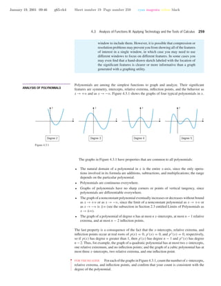
Example 6 Generate or sketch a graph of y =
x3
− x2
− 8
x − 1
.
Solution. Figure 4.3.12 shows a computer-generated graph of
f(x) =
x3
− x2
− 8
x − 1](https://image.slidesharecdn.com/ch04-150306071940-conversion-gate01/85/Ch04-24-320.jpg)
![January 19, 2001 09:46 g65-ch4 Sheet number 25 Page number 265 cyan magenta yellow black
4.3 Analysis of Functions III: Applying Technology and the Tools of Calculus 265
Note that
f(x) = x2
−
8
x − 1
so f(x) ≈ x2
[since 8/(x −1) ≈ 0] as x →−ϱ and as x →+ϱ. Thus, we would expect the
graph to be concave up for large values of x, but the vertical asymptote at x = 1 indicates
that f (x) should be concave down in an interval just to the right of 1, so there should be an
inflection point to the right of x = 1. Also, our sketch indicates a relative minimum to the
left of x = 1. To determine the locations of these features we proceed as follows.
-3 -2 -1 1 2 3 4 5
-15
-10
-5
5
10
15
20
25
x
y
y = x3
– x2
– 8
x – 1
Figure 4.3.12
• Symmetries: There are no symmetries about a vertical axis or about a point.
• x-intercepts: Setting y = 0 leads to solving the equation x3
− x2
− 8 = 0. From
Figure 4.3.12 it appears there is one solution in the interval [2, 3]. Using a solver yields
x ≈ 2.39486.
• y-intercepts: Setting x = 0 yields the y-intercept y = 8.
• Vertical asymptotes: Setting x = 1 would produce a nonzero numerator and a zero
denominator for f (x), so x = 1 is a vertical asymptote.
• Horizontal asymptotes: There are no horizontal asymptotes; however, as noted,
f(x) = x2
−
8
x − 1
so
lim
x →−ϱ
[f (x) − x2
] = lim
x →−ϱ
−
8
x − 1
= 0 and lim
x →+ϱ
[f (x) − x2
] = 0
Thus, f(x) is asymptotic to y = x2
as x →−ϱ and as x →+ϱ.
• Derivatives:
f (x) =
d
dx
x2
−
8
x − 1
= 2x +
8
(x − 1)2
= 2x +
8
(x − 1)2
f (x) =
d
dx
2x +
8
(x − 1)2
= 2 −
16
(x − 1)3
= 2 −
16
(x − 1)3
• Intervals of increase and decrease; relative extrema: f (x) = 0 when
2x = −
8
(x − 1)2
or when 2(x3
− 2x2
+ x + 4) = 2(x + 1)(x2
− 3x + 4) = 0. The only real solution to
this equation is x = −1.
1
0 ∞ + ++++ + + +++++++++–––––
StaDecr Incr Undef Incr
x
Sign of dy/dx
y
–1
The analysis reveals a relative minimum f (−1) = 5 at x = −1.
• Concavity: f (x) = 0 when
2 =
16
(x − 1)3
or when (x − 1)3
= 8. Then x − 1 = 2, so x = 3.
1
∞ – ––––+ + +++++ + +++ +++++0
Concave
up
Concave
down
Concave
up
x
Sign of d2
y/dx2
y
3
The analysis reveals an inflection point at x = 3. The coordinates of the inflection point
are (3, 5).](https://image.slidesharecdn.com/ch04-150306071940-conversion-gate01/85/Ch04-25-320.jpg)
![January 19, 2001 09:46 g65-ch4 Sheet number 30 Page number 270 cyan magenta yellow black
270 The Derivative in Graphing and Applications
neither vertical nor horizontal. To see why, we perform the
division of P(x) by Q(x) to obtain
P(x)
Q(x)
= (ax + b) +
R(x)
Q(x)
where ax +b is the quotient and R(x) is the remainder. Use
the fact that the degree of the remainder R(x) is less than
the degree of the divisor Q(x) to help prove
lim
x →+ϱ
P(x)
Q(x)
− (ax + b) = 0
lim
x →−ϱ
P(x)
Q(x)
− (ax + b) = 0
As illustrated in the accompanying figure, these results tell
us that the graph of the equation y = P(x)/Q(x) “ap-
proaches” the line (an oblique asymptote) y = ax + b as
x →+ϱ or as x →−ϱ.
x
y
y = ax + b
y =
P(x)
Q(x)
(ax + b) –
P(x)
Q(x)
– (ax + b)
P(x)
Q(x)
y =
P(x)
Q(x)
Figure Ex-48
In Exercises 49–53, sketch the graph of the rational function.
Show all vertical, horizontal, and oblique asymptotes (see
Exercise 48).
49.
x2
− 2
x
50.
x2
− 2x − 3
x + 2
51.
(x − 2)3
x2
52.
4 − x3
x2
53. x + 1 −
1
x
−
1
x2
54. Find all values of x where the graph of
y =
2x3
− 3x + 4
x2
crosses its oblique asymptote. (See Exercise 48.)
55. Let f(x) = (x3
+ 1)/x. Show that the graph of y = f(x)
approaches the curve y = x2
asymptotically. Sketch the
graph of y = f(x) showing this asymptotic behavior.
56. Let f(x) = (2 + 3x − x3
)/x. Show that y = f(x) ap-
proaches the curve y = 3 − x2
asymptotically in the sense
described in Exercise 55. Sketch the graph of y = f(x)
showing this asymptotic behavior.
57. A rectangular plot of land is to be fenced off so that the
area enclosed will be 400 ft2
. Let L be the length of fencing
needed and x the length of one side of the rectangle. Show
that L = 2x + 800/x for x > 0, and sketch the graph of L
versus x for x > 0.
58. A box with a square base and open top is to be made from
sheet metal so that its volume is 500 in3
. Let S be the area
of the surface of the box and x the length of a side of the
square base. Show that S = x2
+ 2000/x for x > 0, and
sketch the graph of S versus x for x > 0.
59. The accompanying figure shows a computer-generated
graph of the polynomial y = 0.1x5
(x − 1) using a viewing
window of [−2, 2.5] × [−1, 5]. Show that the choice of the
vertical scale caused the computer to miss important fea-
tures of the graph. Find the features that were missed and
make your own sketch of the graph that shows the missing
features.
60. The accompanying figure shows a computer-generated
graph of the polynomial y = 0.1x5
(x +1)2
using a viewing
window of [−2, 1.5] × [−0.2, 0.2]. Show that the choice
of the vertical scale caused the computer to miss important
features of the graph. Find the features that were missed and
make your own sketch of the graph that shows the missing
features.
-2 -1 1 2
-1
1
2
3
4
5
Generated by Mathematica
Figure Ex-59
Generated by Mathematica
-2 -1 1
-0.2
-0.1
0.1
0.2
Figure Ex-60](https://image.slidesharecdn.com/ch04-150306071940-conversion-gate01/85/Ch04-30-320.jpg)
![January 19, 2001 09:46 g65-ch4 Sheet number 37 Page number 277 cyan magenta yellow black
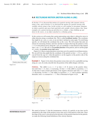
4.4 Rectilinear Motion (Motion Along a Line) 277
4.4.4 THE FREE-FALL MODEL. Suppose that at time t = 0 an object at a height of
s0 above the Earth’s surface is imparted an upward or downward velocity of v0 and
thereafter moves vertically subject only to the force of the Earth’s gravity. If the positive
direction of the s-axis is up, and if the origin is at the surface of the Earth, then at any
time t the height s = s(t) of the object is given by the formula
s = s0 + v0t − 1
2
gt2
(5)
where g is a constant, called the acceleration due to gravity. In this text we will use the
following approximations for g, depending on the units of measurement:
g = 9.8 m/s2
[distance in meters and time in seconds]
g = 32 ft/s2
[distance in feet and time in seconds]
s
s-axis
Height
Earth
Figure 4.4.8
It follows from (5) that the instantaneous velocity and acceleration of an object in free-fall
motion are
v =
ds
dt
= v0 − gt (6)
a =
dv
dt
= −g (7)
••
•
•
•
•
•
•
•
•
•
•
•
•
•
•
•
•
•
•
•
•
•
•
•
•
•
•
•
•
•
•
•
•
•
•
•
•
•
•
•
•
•
•
•
•
•
•
•
•
•
•
•
•
•
REMARK. Because we have chosen the positive direction of the s-axis to be up, a positive
velocity implies an upward motion and a negative velocity a downward motion. Thus, it
makes sense that instantaneous acceleration −g is negative, since an upward-moving object
has positive velocity and negative acceleration, which implies that it is slowing down; and
a downward-moving object has negative velocity and negative acceleration, which implies
that it is speeding up. (It is a little confusing that the positive constant g is called the
acceleration due to gravity in 4.4.4, given that the instantaneous acceleration is actually the
negative constant −g. This mismatch in terminology is caused by the upward orientation
of the s-axis in Figure 4.4.8; had we chosen the positive direction to be down, then the
instantaneous acceleration would have turned out to be g. However, our orientation has the
advantage of allowing us to interpret s as the height of the object.)
Example 7 Nolan Ryan, one of the fastest baseball pitchers of all time, was capable of
throwing a baseball 150 ft/s (over 102 mi/h). During his career, he had the opportunity to
pitch in the Houston Astrodome, home to the Houston Astros Baseball Team from 1965 to
1999. The Astrodome was an indoor stadium with a ceiling 208 ft high. Could Nolan Ryan
have hit the ceiling of the Astrodome if he were capable of giving a baseball an upward
velocity of 100 ft/s from a height of 7 ft?
Nolan Ryan’s rookie baseball card
Solution. Taking g = 32 ft/s2
, v0 = 100 ft/s, and s0 = 7 ft in (5) and (6) yields the
equations
s = 7 + 100t − 16t2
and v = 100 − 32t (8–9)
whose graphs are shown in Figure 4.4.9. It is evident from the graph of s versus t that
the maximum height of the baseball is less than 208 ft, so Ryan could not have hit the
ceiling. However, let us go a step further and determine exactly how high the ball will
go. The maximum height s occurs at the stationary point obtained by solving the equation
ds/dt = 0. However, ds/dt = v, which means that the maximum height occurs when
v = 0, which from (9) can be expressed as
100 − 32t = 0 (10)
Solving this equation yields t = 25/8. To find the height s at this time we substitute this](https://image.slidesharecdn.com/ch04-150306071940-conversion-gate01/85/Ch04-37-320.jpg)
![January 19, 2001 09:46 g65-ch4 Sheet number 39 Page number 279 cyan magenta yellow black
4.4 Rectilinear Motion (Motion Along a Line) 279
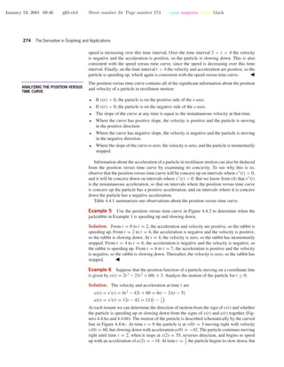
5. Sketch a reasonable graph of s versus t for a mouse that
is trapped in a narrow corridor (an s-axis with the positive
direction to the right) and scurries back and forth as follows.
It runs right with a constant speed of 1.2 m/s for awhile, then
gradually slows down to 0.6 m/s, then quickly speeds up
to 2.0 m/s, then gradually slows to a stop but immediately
reverses direction and quickly speeds up to 1.2 m/s.
6. The accompanying figure shows the graph of s versus t for
an ant that moves along a narrow vertical pipe (an s-axis
with the positive direction up).
(a) When, if ever, is the ant above the origin?
(b) When, if ever, does the ant have velocity zero?
(c) When, if ever, is the ant moving down the pipe?
7. The accompanying figure shows the graph of velocity ver-
sus time for a particle moving along a coordinate line. Make
a rough sketch of the graphs of speed versus time and ac-
celeration versus time.
0 1 2 3 4 5 6 7
t (s)
s
Figure Ex-6
0 1 2 3 4 5 6
-10
-5
0
5
10
15
t (s)
v (m/s)
Figure Ex-7
8. The accompanying figure shows the position versus time
graph for an elevator that ascends 40 m from one stop to the
next.
(a) Estimate the velocity when the elevator is halfway up.
(b) Sketch rough graphs of the velocity versus time curve
and the acceleration versus time curve.
9. The accompanying figure shows the velocity versus time
graph for a test run on a classic Grand Prix GTP. Using this
graph, estimate
(a) the acceleration at 60 mi/h (in units of ft/s2
)
(b) the time at which the maximum acceleration occurs.
[Data from Car and Driver Magazine, October 1990.]
0 5 10 15 20 25
10
20
30
40
Time t (s)
Positions(m)
Figure Ex-8
0 5 10 15 20 25
10
20
30
40
50
60
70
80
90
100
Time t (s)
Velocityv(mi/h)
Figure Ex-9
10. Let s(t) = sin(πt/4) be the position function of a particle
moving along a coordinate line, where s is in meters and t
is in seconds.
(a) Make a table showing the position, velocity, and accel-
eration to two decimal places at times t = 1, 2, 3, 4,
and 5.
(b) At each of the times in part (a), determine whether
the particle is stopped; if it is not, state its direction of
motion.
(c) At each of the times in part (a), determine whether the
particle is speeding up, slowing down, or neither.
In Exercises 11–14, the position function of a particle mov-
ing along a coordinate line is given, where s is in feet and t
is in seconds.
(a) Find the velocity and acceleration functions.
(b) Find the position, velocity, speed, and acceleration at
time t = 1.
(c) At what times is the particle stopped?
(d) When is the particle speeding up? Slowing down?
(e) Find the total distance traveled by the particle from time
t = 0 to time t = 5.
11. s(t) = t3
− 6t2
, t ≥ 0
12. s(t) = t4
− 4t + 2, t ≥ 0
13. s(t) = 3 cos(πt/2), 0 ≤ t ≤ 5
14. s(t) =
t
t2 + 4
, t ≥ 0
15. Let s(t) = t/(t2
+ 5) be the position function of a particle
moving along a coordinate line, where s is in meters and t
is in seconds. Use a graphing utility to generate the graphs
of s(t), v(t), and a(t) for t ≥ 0, and use those graphs where
needed.
(a) Use the appropriate graph to make a rough estimate of
the time at which the particle first reverses the direction
of its motion; and then find the time exactly.
(b) Find the exact position of the particle when it first re-
verses the direction of its motion.
(c) Use the appropriate graphs to make a rough estimate of
the time intervals on which the particle is speeding up
and on which it is slowing down; and then find those
time intervals exactly.
16. Let s(t) = (t2
+ t + 1)/(t2
+ 1) be the position function
of a particle moving along a coordinate line, where s is in
meters and t is in seconds. Use a graphing utility to generate
the graphs of s(t), v(t), and a(t) for t ≥ 0, and use those
graphs where needed.
(a) Use the appropriate graph to make a rough estimate of
the time at which the particle first reverses the direction
of its motion; and then find the time exactly.
(b) Find the exact position of the particle when it first re-
verses the direction of its motion.
(c) Use the appropriate graphs to make a rough estimate of
the time intervals on which the particle is speeding up](https://image.slidesharecdn.com/ch04-150306071940-conversion-gate01/85/Ch04-39-320.jpg)
![January 19, 2001 09:46 g65-ch4 Sheet number 40 Page number 280 cyan magenta yellow black
280 The Derivative in Graphing and Applications
and on which it is slowing down; and then find those
time intervals exactly.
In Exercises 17–22, the position function of a particle moving
along a coordinate line is given. Use the method of Example
6 to analyze the motion of the particle for t ≥ 0, and give a
schematic picture of the motion (as in Figure 4.4.6).
17. s = −3t + 2 18. s = t3
− 6t2
+ 9t + 1
19. s = t3
− 9t2
+ 24t 20. s = t +
9
t + 1
21. s =
cos t, 0 ≤ t ≤ 2π
1, t > 2π
22. s =
√
t(4 − 4t + 2t2
)
23. Let s(t) = 5t2
− 22t be the position function of a particle
moving along a coordinate line, where s is in feet and t is
in seconds.
(a) Find the maximum speed of the particle during the time
interval 1 ≤ t ≤ 3.
(b) When, during the time interval 1 ≤ t ≤ 3, is the parti-
cle farthest from the origin? What is its position at that
instant?
24. Let s = 100/(t2
+ 12) be the position function of a particle
moving along a coordinate line, where s is in feet and t is in
seconds. Find the maximum speed of the particle for t ≥ 0,
and find the direction of motion of the particle when it has
its maximum speed.
In Exercises 25–29, assume that the free-fall model applies
and that the positive direction is up, so that Formulas (5), (6),
and (7) can be used. In those problems stating that an object is
“dropped” or “released from rest,” you should interpret that
to mean that the initial velocity of the object is zero. Take
g = 32 ft/s2
or g = 9.8 m/s2
, depending on the units.
25. A wrench is accidentally dropped at the top of an elevator
shaft in a tall building.
(a) How many meters does the wrench fall in 1.5 s?
(b) What is the velocity of the wrench at that time?
(c) How long does it take for the wrench to reach a speed
of 12 m/s?
(d) How long does it take for the wrench to fall 100 m?
26. In 1939, Joe Sprinz of the San Francisco Seals Baseball Club
attempted to catch a ball dropped from a blimp at a height of
800 ft (for the purpose of breaking the record for catching a
ball dropped from the greatest height set the preceding year
by members of the Cleveland Indians).
(a) How long does it take for a ball to drop 800 ft?
(b) What is the velocity of a ball in miles per hour after an
800-ft drop (88 ft/s = 60 mi/h)?
[Note: As a practical matter, it is unrealistic to ignore wind
resistance in this problem; however, even with the slowing
effect of wind resistance, the impact of the ball slammed
Sprinz’s glove hand into his face, fractured his upper jaw in
12 places, broke five teeth, and knocked him unconscious.
He dropped the ball!]
27. A projectile is launched upward from ground level with an
initial speed of 60 m/s.
(a) How long does it take for the projectile to reach its
highest point?
(b) How high does the projectile go?
(c) How long does it take for the projectile to drop back to
the ground from its highest point?
(d) What is the speed of the projectile when it hits the
ground?
28. (a) UsetheresultsinExercise27tomakeaconjectureabout
the relationship between the initial and final speeds of
a projectile that is launched upward from ground level
and returns to ground level.
(b) Prove your conjecture.
29. In Example 7, how fast would Nolan Ryan have to throw a
ball upward from a height of 7 feet in order to hit the ceiling
of the Astrodome?
30. The free-fall formulas (5) and (6) can be combined and
rearranged in various useful ways. Derive the following
variations of those formulas.
(a) v2
= v2
0 − 2g(s − s0) (b) s = s0 + 1
2
(v0 + v)t
(c) s = s0 + vt + 1
2
gt2
31. A rock, dropped from an unknown height, strikes the ground
with a speed of 24 m/s. Use the formula in part (a) of Ex-
ercise 30 to find the unknown height.
32. A rock thrown downward with an unknown initial velocity
from a height of 1000 ft reaches the ground in 5 s. Use the
formula in part (c) of Exercise 30 to find the velocity of the
rock when it hits the ground.
33. (a) A ball is thrown upward from a height s0 with an ini-
tial velocity of v0. Use the formula in part (a) of Exer-
cise 30 to show that the maximum height of the ball is
smax = s0 + v2
0
/2g.
(b) Use this result to solve Exercise 29.
34. Let s = t3
− 6t2
+ 1.
(a) Find s and v when a = 0.
(b) Find s and a when v = 0.
35. Let s =
√
2t2 + 1 be the position function of a particle
moving along a coordinate line.
(a) Use a graphing utility to generate the graph of v versus
t, and make a conjecture about the velocity of the par-
ticle as t →+ϱ.
(b) Check your conjecture by finding lim
t →+ϱ
v.
36. (a) Use the chain rule to show that for a particle in rectilin-
ear motion a = v(dv/ds).
(b) Let s =
√
3t + 7, t ≥ 0. Find a formula for v in terms
of s and use the equation in part (a) to find the acceler-
ation when s = 5.
37. Suppose that the position functions of two particles, P1 and
P2, in motion along the same line are
s1 = 1
2
t2
− t + 3 and s2 = −1
4
t2
+ t + 1
respectively, for t ≥ 0.](https://image.slidesharecdn.com/ch04-150306071940-conversion-gate01/85/Ch04-40-320.jpg)
![January 19, 2001 09:46 g65-ch4 Sheet number 41 Page number 281 cyan magenta yellow black
4.5 Absolute Maxima and Minima 281
(a) Prove that P1 and P2 do not collide.
(b) How close can P1 and P2 get to one another?
(c) During what intervals of time are they moving in oppo-
site directions?
38. Let sA = 15t2
+10t +20 and sB = 5t2
+40t, t ≥ 0, be the
position functions of cars A and B that are moving along
parallel straight lanes of a highway.
(a) How far is car A ahead of car B when t = 0?
(b) At what instants of time are the cars next to one another?
(c) At what instant of time do they have the same velocity?
Which car is ahead at this instant?
39. Prove that a particle is speeding up if the velocity and accel-
eration have the same sign, and slowing down if they have
opposite signs. [Hint: Let r(t) = |v(t)| and find r (t) using
the chain rule.]
4.5 ABSOLUTE MAXIMA AND MINIMA
At the beginning of Section 4.2 we observed that if the graph of a function f is viewed
as a two-dimensional mountain range (Figure 4.2.1), then the relative maxima and
minima correspond to the tops of the hills and the bottoms of the valleys; that is, they
are the high and low points in their immediate vicinity. In this section we will be con-
cerned with the more encompassing problem of finding the highest and lowest points
over the entire mountain range, that is, we will be looking for the top of the highest
hill and the bottom of the deepest valley. In mathematical terms, we will be looking for
the largest and smallest values of a function over an interval.
• • • • • • • • • • • • • • • • • • • • • • • • • • • • • • • • • • • • • •
ABSOLUTE EXTREMA
We will be concerned here with finding the largest and smallest values of a function over a
finite or infinite interval I. We begin with some terminology.
4.5.1 DEFINITION. A function f is said to have an absolute maximum on an interval
I at x0 if f(x0) is the largest value of f on I; that is, f(x0) ≥ f(x) for all x in I.
Similarly, f is said to have an absolute minimum on I at x0 if f(x0) is the smallest value
of f on I; that is, f(x0) ≤ f(x) for all x in I. If f has either an absolute maximum or
absolute minimum on I at x0, then f is said to have an absolute extremum on I at x0.
As illustrated in Figure 4.5.1, there is no guarantee that a function f will have absolute
extrema on a given interval.
• • • • • • • • • • • • • • • • • • • • • • • • • • • • • • • • • • • • • •
EXISTENCE OF ABSOLUTE
EXTREMA
The remainder of this section will focus on the following problem.
4.5.2 PROBLEM.
(a) Determine whether a function f has any absolute extrema on a given interval I.
(b) If there are absolute extrema, determine where they occur and what the absolute
maximum and minimum values are.
Parts (a)–(e) of Figure 4.5.1 show that a continuous function may or may not have absolute
maxima or minima on an infinite interval or on a finite open interval. However, the following
theorem shows that a continuous function must have both an absolute maximum and an
absolute minimum on every finite closed interval [see part ( f ) of Figure 4.5.1].
4.5.3 THEOREM (Extreme-Value Theorem). If a function f is continuous on a finite
closed interval [a, b], then f has both an absolute maximum and an absolute minimum
on [a, b].](https://image.slidesharecdn.com/ch04-150306071940-conversion-gate01/85/Ch04-41-320.jpg)
![January 19, 2001 09:46 g65-ch4 Sheet number 42 Page number 282 cyan magenta yellow black
282 The Derivative in Graphing and Applications
x
y
f has no absolute
extrema on
(–∞, +∞).
x
y
f has an absolute
minimum but no
absolute maximum
on (–∞, +∞).
x
y
f has an absolute
maximum and
minimum on
(–∞, +∞).
(a) (b) (c)
x
y
f has no absolute
extrema on (a, b).
x
y
x
y
f has an absolute
maximum and
minimum on (a, b).
f has an absolute
maximum and
minimum on [a, b].
(d) (e) ( f)
( (
a b
( (
a b
[ [
a b
Figure 4.5.1
••
•
•
•
•
•
•
•
•
•
•
•
•
•
•
•
•
•
•
•
•
•
•
•
•
•
•
•
•
•
•
•
FOR THE READER. Although the proof of this theorem is too difficult to include here,
you should be able to convince yourself of its validity with a little experimentation—try
graphing various continuous functions over the interval [0, 1], and convince yourself that
there is no way to avoid having a highest and lowest point on the graph. As a physical
analogy, if you imagine the graph to be a roller coaster track starting at x = 0 and ending at
x = 1, the roller coaster will have to pass through a highest point and a lowest point during
the trip.
The function f (x) = 2x + 1 is continuous everywhere, so the Extreme-Value Theorem
guarantees that f (x) has both an absolute maximum and an absolute minimum on every
finite closed interval. For example, on the interval [0, 3], the absolute minimum occurs at
x = 0 and the absolute maximum occurs at x = 3. The absolute minimum and maximum
values for f (x) on [0, 3] are f (0) = 1 and f (3) = 7, respectively (Figure 4.5.2).
3
1
0
7
x
y
f(x) = 2x + 1
Figure 4.5.2
x
y
a b
No absolute
minimum
No absolute
maximum
Figure 4.5.3
3x0
x1
1
0
7
x
y
f(x) = 2x + 1
Figure 4.5.4
The hypotheses of the Extreme-Value Theorem are essential. Figure 4.5.3 shows the
graph of a function that is defined on a closed interval [a, b] but fails to be continuous on
that interval. This function has neither an absolute maximum nor an absolute minimum on
the interval [a, b]. If f is continuous on an interval that is not both closed and finite, then
we could encounter situations such as those in Figure 4.5.1.
To illustrate further, consider again the function f (x) = 2x + 1, but now for values of
x in the half-open interval [0, 3). The function f has an absolute minimum value of 1 at
x = 0 in the interval [0, 3). However, for any number x0 in [0, 3) that we might choose
as a candidate for the location of an absolute maximum, we can find another number, say
x1 = (x0 + 3)/2, also in [0, 3), with f (x1) > f (x0) (Figure 4.5.4). Thus, for any particular
value of f (x) on [0, 3), we can find a larger value of the function on this interval; that is,
f does not attain an absolute maximum value on [0, 3).](https://image.slidesharecdn.com/ch04-150306071940-conversion-gate01/85/Ch04-42-320.jpg)
![January 19, 2001 09:46 g65-ch4 Sheet number 43 Page number 283 cyan magenta yellow black
4.5 Absolute Maxima and Minima 283
• • • • • • • • • • • • • • • • • • • • • • • • • • • • • • • • • • • • • •
FINDING ABSOLUTE EXTREMA ON
FINITE CLOSED INTERVALS
The Extreme-Value Theorem is an example of what mathematicians call an existence theo-
rem. Such theorems state conditions under which certain objects exist, in this case absolute
extrema. However, knowing that an object exists and finding it are two separate things.
We will now address methods for determining the locations of absolute extrema under the
conditions of the Extreme-Value Theorem.
If f is continuous on the finite closed interval [a, b], then the absolute extrema of f
can occur either at the endpoints of the interval or inside on the open interval (a, b). If the
absolute extrema happen to fall inside, then the following theorem tells us that they must
occur at critical numbers of f .
4.5.4 THEOREM. If f has an absolute extremum on an open interval (a, b), then it
must occur at a critical number of f .
Proof. If f has an absolute maximum on (a, b) at x0, then f(x0) is also a relative maximum
for f ; for if f(x0) is the largest value of f on all of (a, b), then f(x0) is certainly the largest
value for f in the immediate vicinity of x0. Thus, x0 is a critical number of f by Theorem
4.2.2. The proof for absolute minima is similar.
•••• REMARK. Theorem 4.5.4 is also valid for functions on infinite open intervals.
It follows from this theorem, that if f is continuous on the finite closed interval [a, b],
then the absolute extrema occur either at the endpoints of the interval or at critical numbers
inside the interval (Figure 4.5.5). Thus, we can use the following procedure to find the
absolute extrema of a continuous function on a finite closed interval [a, b].
a x0 ba x0 ba b
Absolute maximum
occurs at an endpoint.
Absolute maximum occurs
in the open interval (a, b) at
a value x0 where f ′(x0) = 0.
Absolute maximum occurs
in the open interval (a, b)
at a value x0 where f is
not differentiable.
x
y
x
y
x
y
Figure 4.5.5
A Procedure for Finding the Absolute Extrema of a Continuous Function f
on a Finite Closed Interval [a, b].
Step 1. Find the critical numbers of f in (a, b).
Step 2. Evaluate f at all the critical numbers and at the endpoints a and b.
Step 3. The largest of the values in Step 2 is the absolute maximum value of
f on [a, b] and the smallest value is the absolute minimum.](https://image.slidesharecdn.com/ch04-150306071940-conversion-gate01/85/Ch04-43-320.jpg)
![January 19, 2001 09:46 g65-ch4 Sheet number 44 Page number 284 cyan magenta yellow black
284 The Derivative in Graphing and Applications
Example 1 Find the absolute maximum and minimum values of f(x) = 2x3
−15x2
+36x
on the interval [1, 5], and determine where these values occur.
Solution. Since f is continuous and differentiable everywhere, the absolute extrema must
occur either at endpoints of the interval or at solutions to the equation f (x) = 0 in the open
interval (1, 5). The equation f (x) = 0 can be written as
6x2
− 30x + 36 = 6(x2
− 5x + 6) = 6(x − 2)(x − 3) = 0
Thus, there are stationary points at x = 2 and at x = 3. Evaluating f at the endpoints, at
x = 2, and at x = 3 yields
f(1) = 2(1)3
− 15(1)2
+ 36(1) = 23
f(2) = 2(2)3
− 15(2)2
+ 36(2) = 28
f(3) = 2(3)3
− 15(3)2
+ 36(3) = 27
f(5) = 2(5)3
− 15(5)2
+ 36(5) = 55
from which we conclude that an absolute minimum of f on [1, 5] is 23, occurring at x = 1,
and the absolute maximum of f on [1, 5] is 55, occurring at x = 5. This is consistent with
the graph of f in Figure 4.5.6.
[1, 5] × [20, 55]
xScl = 1, yScl = 10
y = 2x3
– 15x2
+ 36x
Figure 4.5.6
Example 2 Find the absolute extrema of f(x) = 6x4/3
− 3x1/3
on the interval [−1, 1],
and determine where these values occur.
Solution. Note that f is continuous everywhere and therefore the Extreme-Value The-
orem guarantees that f has a maximum and a minimum value in the interval [−1, 1].
Differentiating, we obtain
f (x) = 8x1/3
− x−2/3
= x−2/3
(8x − 1) =
8x − 1
x2/3
Thus, f (x) = 0 at x = 1
8
, and f (x) is undefined at x = 0. Evaluating f at these
critical numbers and endpoints yields Table 4.5.1, from which we conclude that an absolute
minimum value of −9
8
occurs at x = 1
8
, and an absolute maximum value of 9 occurs at
x = −1.
Table 4.5.1
–1
9
0
0
1
3
x
f(x)
1
8
9
8
–
• • • • • • • • • • • • • • • • • • • • • • • • • • • • • • • • • • • • • •
ABSOLUTE EXTREMA ON INFINITE
INTERVALS
We observed earlier that a continuous function may or may not have absolute extrema on
an infinite interval (see Figure 4.5.1). However, certain conclusions about the existence of
absolute extrema of a continuous function f on (−ϱ, +ϱ) can be drawn from the behavior
of f(x) as x →−ϱ and as x →+ϱ (Table 4.5.2).
Table 4.5.2
f has an absolute minimum
but no absolute maximum
on (−∞, +∞).
f has an absolute maximum
but no absolute minimum
on (−∞, +∞).
f has neither an absolute
maximum nor an absolute
minimum on (−∞, +∞).
f has neither an absolute
maximum nor an absolute
minimum on (−∞, +∞).
limits
graph
conclusion if
f is continuous
everywhere
lim f(x) = +∞
x →−∞
lim f(x) = +∞
x →+∞
lim f(x) = –∞
x →−∞
lim f(x) = –∞
x →+∞
lim f(x) = –∞
x →−∞
lim f(x) = +∞
x →+∞
lim f(x) = +∞
x →−∞
lim f(x) = –∞
x →+∞
x
y
x
y
x
y
x
y](https://image.slidesharecdn.com/ch04-150306071940-conversion-gate01/85/Ch04-44-320.jpg)
![January 19, 2001 09:46 g65-ch4 Sheet number 45 Page number 285 cyan magenta yellow black
4.5 Absolute Maxima and Minima 285
Example 3 What can you say about the existence of absolute extrema on (−ϱ, +ϱ) for
polynomials?
Solution. If p(x) is a polynomial of odd degree, then
lim
x →+ϱ
p(x) and lim
x →−ϱ
p(x) (1)
have opposite signs (one is +ϱ and the other is −ϱ), so there are no absolute extrema. On
the other hand, if p(x) has even degree, then the limits in (1) have the same sign (both +ϱ
or both −ϱ). If the leading coefficient is positive, then both limits are +ϱ, and there is an
absolute minimum but no absolute maximum; if the leading coefficient is negative, then
both limits are −ϱ, and there is an absolute maximum but no absolute maximum.
Example 4 Determine by inspection whether p(x) = 3x4
+4x3
has any absolute extrema.
If so, find them and state where they occur.
Solution. Since p(x) has even degree and the leading coefficient is positive, p(x)→+ϱ
as x →±ϱ. Thus, there is an absolute minimum but no absolute maximum. From Theorem
4.5.4 [applied to the interval (−ϱ, +ϱ)], the absolute minimum must occur at a critical
number of p. Since p is differentiable everywhere, we can find all critical numbers by
solving the equation p (x) = 0. This equation is
12x3
+ 12x2
= 12x2
(x + 1) = 0
from which we conclude that the critical numbers are x = 0 and x = −1. Evaluating p at
these critical numbers yields
p(0) = 0 and p(−1) = −1
Therefore, p has an absolute minimum of −1 at x = −1 (Figure 4.5.7).
p(x) = 3x4
+ 4x3
-2 2
3
x
y
Figure 4.5.7
• • • • • • • • • • • • • • • • • • • • • • • • • • • • • • • • • • • • • •
ABSOLUTE EXTREMA ON OPEN
INTERVALS
We know that a continuous function may or may not have absolute extrema on an open
interval. However, certain conclusions about the existence of absolute extrema of a contin-
uous function f on a finite open interval (a, b) can be drawn from the behavior of f(x) as
x →a+
and as x →b−
(Table 4.5.3). Similar conclusions can be drawn for intervals of the
form (−ϱ, b) or (a, +ϱ).
Table 4.5.3
a b
a b
a b
a b
f has an absolute
minimum but no absolute
maximum on (a, b).
f has an absolute
maximum but no absolute
minimum on (a, b).
f has neither an absolute
maximum nor an absolute
minimum on (a, b).
f has neither an absolute
maximum nor an absolute
minimum on (a, b).
limits
graph
conclusion if
f is continuous
on (a, b)
lim f(x) = +∞
x→a+
lim f(x) = +∞
x→b–
lim f(x) = –∞
x→a+
lim f(x) = –∞
x→b–
lim f(x) = –∞
x→a+
lim f(x) = +∞
x→b–
lim f(x) = +∞
x→a+
lim f(x) = –∞
x→b–
x x
x
x
Example 5 Determine whether the function
f(x) =
1
x2 − x
has any absolute extrema on the interval (0, 1). If so, find them and state where they occur.](https://image.slidesharecdn.com/ch04-150306071940-conversion-gate01/85/Ch04-45-320.jpg)
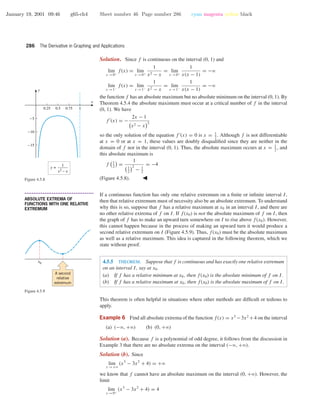
![January 19, 2001 09:46 g65-ch4 Sheet number 47 Page number 287 cyan magenta yellow black
4.5 Absolute Maxima and Minima 287
is not infinite, so there is a possibility that f may have an absolute minimum on this interval.
In this case it would have to occur at a stationary point, which suggests that we look for
solutions of the equation f (x) = 0. But,
f (x) = 3x2
− 6x = 3x(x − 2)
so f has critical numbers x = 0 and x = 2. However, the only critical number inside the
interval (0, +ϱ) is at x = 2. Thus, Theorem 4.5.5 is applicable here. Since
f (x) = 6x − 6
we have f (2) = 6 > 0, so a relative minimum occurs at x = 2 by the second derivative
test. Thus, f(x) has an absolute minimum at x = 2, and this absolute minimum is f(2) = 0
(Figure 4.5.10).
1 2 3 4 5
2
4
6
8
10
x
y
f(x) = x3
– 3x2
+ 4, x > 0
Figure 4.5.10
• • • • • • • • • • • • • • • • • • • • • • • • • • • • • • • • • • • • • •
ABSOLUTE EXTREMA AND
PARAMETRIC CURVES
Suppose that a curve C is given parametrically by the equations
x = f(t), y = g(t) (a ≤ t ≤ b)
where f and g are continuous on the finite closed interval [a, b]. It follows from the
Extreme-Value Theorem that f(t) and g(t) have absolute maxima and absolute minima for
a ≤ t ≤ b; this means that a particle moving along the curve cannot move away from the
origin indefinitely—there must be a smallest and largest x-coordinate and a smallest and
largest y-coordinate. Geometrically, the entire curve is contained within a box determined
by these smallest and largest coordinates.
Example 7 Suppose that the equations of motion for a paper airplane during its first 10
seconds of flight are
x = t − 3 sin t, y = 4 − 3 cos t (0 ≤ t ≤ 10)
What are the highest and lowest points in the trajectory, and when is the airplane at those
points?
Solution. The trajectory, pictured in Figure 4.5.11, is shown in more detail in Figure 1.8.2.
We want to find the absolute maximum and minimum values of y over the time interval
[0, 10] and the values of t for which these absolute extrema occur. The absolute extrema
must occur either at the endpoints of the closed interval [0, 10] or at critical numbers in the
open interval (0, 10). To find the critical numbers, we must solve the equation dy/dt = 0,
which is
3 sin t = 0
Thus, there are critical numbers in the interval (0, 10) at t = π, 2π, and 3π. Evaluating
y = 4 − 3 cos t at the endpoints and the critical numbers yields
-2 2 4 6 8 10 12
2
4
6
8
x
y
Figure 4.5.11](https://image.slidesharecdn.com/ch04-150306071940-conversion-gate01/85/Ch04-47-320.jpg)
![January 19, 2001 09:46 g65-ch4 Sheet number 48 Page number 288 cyan magenta yellow black
288 The Derivative in Graphing and Applications
y = 4 − 3 cos 0 = 4 − 3 = 1
y = 4 − 3 cos π = 4 − (−3) = 7
y = 4 − 3 cos 2π = 4 − 3 = 1
y = 4 − 3 cos 3π = 4 − (−3) = 7
y = 4 − 3 cos 10 ≈ 6.517
Thus, a high point of y = 7 is reached at times t = π and t = 3π, and a low point of y = 1
is reached at times t = 0 and t = 2π. This is consistent with Figure 1.8.2.
EXERCISE SET 4.5 Graphing Calculator C CAS
• • • • • • • • • • • • • • • • • • • • • • • • • • • • • • • • • • • • • • • • • • • • • • • • • • • • • • • • • • • • • • • • • • • • • • • • • • • • • • • • • • • • • • • • • • • • • • • • • • • • • • • • • • • • • •
In Exercises 1–2, use the graph to find x-coordinates of the
relative extrema and absolute extrema of f on [0, 7].
1.
1
1
x
y
y = f(x)
2.
1
1
x
y
y = f(x)
3. In each part, sketch the graph of a continuous function f
with the stated properties on the interval [0, 10].
(a) f has an absolute minimum at x = 0 and an absolute
maximum at x = 10.
(b) f has an absolute minimum at x = 2 and an absolute
maximum at x = 7.
(c) f has a relative minima at x = 1 and x = 8, has relative
maxima at x = 3 and x = 7, has an absolute minimum
at x = 5, and has an absolute maximum at x = 10.
4. In each part, sketch the graph of a continuous function f
with the stated properties on the interval (−ϱ, +ϱ).
(a) f has no relative extrema or absolute extrema.
(b) f has an absolute minimum at x = 0 but no absolute
maximum.
(c) f has an absolute maximum at x = −5 and an absolute
minimum at x = 5.
In Exercises 5–14, find the absolute maximum and minimum
values of f on the given closed interval, and state where those
values occur.
5. f(x) = 4x2
− 4x + 1; [0, 1]
6. f(x) = 8x − x2
; [0, 6]
7. f(x) = (x − 1)3
; [0, 4]
8. f(x) = 2x3
− 3x2
− 12x; [−2, 3]
9. f(x) =
3x
4x2 + 1
; [−1, 1]
10. f(x) = x2
+ x
2/3
; [−2, 3]
11. f(x) = x − tan x; [−π/4, π/4]
12. f(x) = sin x − cos x; [0, π]
13. f(x) = 1 + |9 − x2
|; [−5, 1]
14. f(x) = |6 − 4x|; [−3, 3]
In Exercises 15–22, find the absolute maximum and min-
imum values of f , if any, on the given interval, and state
where those values occur.
15. f(x) = x2
− 3x − 1; (−ϱ, +ϱ)
16. f(x) = 3 − 4x − 2x2
; (−ϱ, +ϱ)
17. f(x) = 4x3
− 3x4
; (−ϱ, +ϱ)
18. f(x) = x4
+ 4x; (−ϱ, +ϱ)
19. f(x) = x3
− 3x − 2; (−ϱ, +ϱ)
20. f(x) = x3
− 9x + 1; (−ϱ, +ϱ)
21. f(x) =
x2
x + 1
; (−5, −1) 22. f(x) =
x + 3
x − 3
; [−5, 5]
In Exercises 23–32, use a graphing utility to estimate the ab-
solute maximum and minimum values of f , if any, on the
stated interval, and then use calculus methods to find the ex-
act values.
23. f(x) = x2
− 1
2
; (−ϱ, +ϱ)
24. f(x) = (x − 1)2
(x + 2)2
; (−ϱ, +ϱ)
25. f(x) = x2/3
(20 − x); [−1, 20]
26. f(x) =
x
x2 + 2
; [−1, 4]
27. f(x) = 1 +
1
x
; (0, +ϱ)
28. f(x) =
x
x2 + 1
; [0, +ϱ)
29. f(x) = 2 sec x − tan x; [0, π/4]
30. f(x) = sin2
x + cos x; [−π, π]](https://image.slidesharecdn.com/ch04-150306071940-conversion-gate01/85/Ch04-48-320.jpg)
![January 19, 2001 09:46 g65-ch4 Sheet number 49 Page number 289 cyan magenta yellow black
4.5 Absolute Maxima and Minima 289
31. f(x) = sin(cos x); [0, 2π]
32. f(x) = cos(sin x); [0, π]
33. Find the absolute maximum and minimum values of
f(x) =
4x − 2, x < 1
(x − 2)(x − 3), x ≥ 1
on 1
2
, 7
2
.
34. Let f(x) = x2
+ px + q. Find the values of p and q such
that f(1) = 3 is an extreme value of f on [0, 2]. Is this
value a maximum or minimum?
If f is a periodic function, then the locations of all absolute
extrema on the interval (−ϱ, +ϱ) can be obtained by finding
the locations of the absolute extrema for one period and using
the periodicity to locate the rest. Use this idea in Exercises 35
and 36 to find the absolute maximum and minimum values
of the function, and state the x-values at which they occur.
35. f(x) = 2 sin 2x + sin 4x 36. f(x) = 3 cos
x
3
+ 2 cos
x
2
One way of proving that f(x) ≤ g(x) for all x in a given
interval is to show that 0 ≤ g(x) − f(x) for all x in the inter-
val; and one way of proving the latter inequality is to show
that the absolute minimum value of g(x) − f(x) on the in-
terval is nonnegative. Use this idea to prove the inequalities
in Exercises 37 and 38.
37. Prove that sin x ≤ x for all x in the interval [0, 2π].
38. Prove that cos x ≥ 1−(x2/2) for all x in the interval [0, 2π].
39. What is the smallest possible slope for a tangent to the graph
of the equation y = x3
− 3x2
+ 5x?
40. (a) Show that
f(x) =
64
sin x
+
27
cos x
has a minimum value but no maximum value on the
interval (0, π/2).
(b) Find the minimum value.
C 41. Show that the absolute minimum value of
f(x) = x2
+
16x2
(8 − x)2
, x > 8
occurs at x = 4(2 + 3√
2 ) by using a CAS to find f (x) and
to solve the equation f (x) = 0.
C 42. Suppose that A and B denote any two positive real numbers.
Use a CAS to determine the maximum value of the function
f(x) = A cos x + B sin x in terms of A and B.
43. It can be proved that if f is differentiable on (a, b) and L
is a line that does not intersect the curve y = f(x) over an
interval (a, b), then the points at which the curve is closest
to or farthest from the line L, if any, occur at points where
the tangent line to the curve is parallel to L (see the ac-
companying figure). Use this result to find the points on the
graph of y = −x2
that are closest to and farthest from the
line y = 2 − x for −1 ≤ x ≤ 3
2
.
x
y
y = f(x)
L
Perpendicular
distance
Figure Ex-43
44. Use the idea discussed in Exercise 43 to find the coordinates
of all points on the graph of y = x3
closest to and farthest
from the line y = 4
3
x − 1 for −1 ≤ x ≤ 1.
45. Suppose that the equations of motion of a paper airplane
during the first 12 seconds of flight are
x = t − 2 sin t, y = 2 − 2 cos t (0 ≤ t ≤ 12)
What are the highest and lowest points in the trajectory, and
when is the airplane at those points?
46. The accompanying figure shows the path of a fly whose
equations of motion are
x =
cos t
2 + sin t
, y = 3 + sin(2t) − 2 sin2
t (0 ≤ t ≤ 2π)
(a) How high and low does it fly?
(b) How far left and right of the origin does it fly?
x
y
Figure Ex-46
47. Let f(x) = ax2
+ bx + c, where a > 0. Prove that
f(x) ≥ 0 for all x if and only if b2
− 4ac ≤ 0. [Hint:
Find the minimum of f(x).]
48. Prove Theorem 4.5.4 in the case where the extreme value is
a minimum.](https://image.slidesharecdn.com/ch04-150306071940-conversion-gate01/85/Ch04-49-320.jpg)
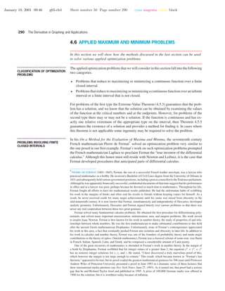
![January 19, 2001 09:46 g65-ch4 Sheet number 51 Page number 291 cyan magenta yellow black
4.6 Applied Maximum and Minimum Problems 291
Example 1 A garden is to be laid out in a rectangular area and protected by a chicken wire
fence. What is the largest possible area of the garden if only 100 running feet of chicken
wire is available for the fence?
Solution. Let
x = length of the rectangle (ft)
y = width of the rectangle (ft)
A = area of the rectangle (ft2
)
Then
A = xy (1)
Since the perimeter of the rectangle is 100 ft, the variables x and y are related by the equation
2x + 2y = 100 or y = 50 − x (2)
(See Figure 4.6.1.) Substituting (2) in (1) yields
A = x(50 − x) = 50x − x2
(3)
Because x represents a length it cannot be negative, and because the two sides of length x
cannot have a combined length exceeding the total perimeter of 100 ft, the variable x must
satisfy
0 ≤ x ≤ 50 (4)
Thus, we have reduced the problem to that of finding the value (or values) of x in [0, 50],
for which A is maximum. Since A is a polynomial in x, it is continuous on [0, 50], and so
the maximum must occur at an endpoint of this interval or at a critical number.
x
x
y y
Perimeter
2x + 2y = 100
Figure 4.6.1
From (3) we obtain
dA
dx
= 50 − 2x
Setting dA/dx = 0 we obtain
50 − 2x = 0
or x = 25. Thus, the maximum occurs at one of the values
x = 0, x = 25, x = 50
Substituting these values in (3) yields Table 4.6.1, which tells us that the maximum area of
625 ft2
occurs at x = 25, which is consistent with the graph of (3) in Figure 4.6.2. From (2)
the corresponding value of y is 25, so the rectangle of perimeter 100 ft with greatest area is
a square with sides of length 25 ft.
Table 4.6.1
0
0
25
625
50
0
x
A
5 10 15 20 25 30 35 40 45 50
100
200
300
400
500
600
700
x (ft)
A (ft2
)
Figure 4.6.2
••
•
•
•
•
•
•
•
•
•
•
•
•
•
•
•
•
•
•
•
•
•
•
•
•
•
•
•
REMARK. In this example we included x = 0 and x = 50 as possible values for x, even
though both values lead to rectangles with two sides of length zero. Whether or not these
values should be allowed will depend on our objective in the problem. If we view this purely
as a mathematical problem, then there is nothing wrong with allowing sides of length zero.
However, if we view this as an applied problem in which the rectangle will be formed from
physical material, then these values should be excluded.](https://image.slidesharecdn.com/ch04-150306071940-conversion-gate01/85/Ch04-51-320.jpg)
![January 19, 2001 09:46 g65-ch4 Sheet number 52 Page number 292 cyan magenta yellow black
292 The Derivative in Graphing and Applications
Example 1 illustrates the following five-step procedure that can be used for solving many
applied maximum and minimum problems.
Step 1. Draw an appropriate figure and label the quantities relevant to the
problem.
Step 2. Find a formula for the quantity to be maximized or minimized.
Step 3. Using the conditions stated in the problem to eliminate variables,
express the quantity to be maximized or minimized as a function of
one variable.
Step 4. Find the interval of possible values for this variable from the physical
restrictions in the problem.
Step 5. If applicable, use the techniques of the preceding section to obtain
the maximum or minimum.
Example 2 An open box is to be made from a 16-inch by 30-inch piece of cardboard
by cutting out squares of equal size from the four corners and bending up the sides (Fig-
ure 4.6.3). What size should the squares be to obtain a box with the largest volume?
x
x
x
x
x
x
x
x
16 in
30 in
16 – 2x
30 – 2x
x
(b)(a)
Figure 4.6.3
Solution. For emphasis, we explicitly list the steps of the five-step problem-solving pro-
cedure given above as an outline for the solution of this problem. (In later examples we will
follow these guidelines implicitly.)
• Step 1: Figure 4.6.3a illustrates the cardboard piece with squares removed from its
corners. Let
x = length (in inches) of the sides of the squares to be cut out
V = volume (in cubic inches) of the resulting box
• Step 2: Because we are removing a square of side x from each corner, the resulting box
will have dimensions 16 − 2x by 30 − 2x by x (Figure 4.6.3b). Since the volume of a
box is the product of its dimensions, we have
V = (16 − 2x)(30 − 2x)x = 480x − 92x2
+ 4x3
(5)
• Step 3: Note that our expression for volume is already in terms of the single variable x.
• Step 4: The variable x in (5) is subject to certain restrictions. Because x represents a
length, it cannot be negative, and because the width of the cardboard is 16 inches, we
cannot cut out squares whose sides are more than 8 inches long. Thus, the variable x in
(5) must satisfy
0 ≤ x ≤ 8
and hence we have reduced our problem to finding the value (or values) of x in the
interval [0, 8] for which (5) is a maximum.](https://image.slidesharecdn.com/ch04-150306071940-conversion-gate01/85/Ch04-52-320.jpg)
![January 19, 2001 09:46 g65-ch4 Sheet number 53 Page number 293 cyan magenta yellow black
4.6 Applied Maximum and Minimum Problems 293
• Step 5: From (5) we obtain
dV
dx
= 480 − 184x + 12x2
= 4(120 − 46x + 3x2
)
= 4(x − 12)(3x − 10)
Setting dV /dx = 0 yields
x = 10
3
and x = 12
Since x = 12 falls outside the interval [0, 8], the maximum value of V occurs either
at the critical number x = 10
3
or at the endpoints x = 0, x = 8. Substituting these
values into (5) yields Table 4.6.2, which tells us that the greatest possible volume
V = 19600
27
in3
≈ 726 in3
occurs when we cut out squares whose sides have length 10
3
inches. This is consistent with the graph of (5) shown in Figure 4.6.4.
Table 4.6.2
0
0
8
0
x
V
10
3
19600
27
≈ 726
1 2 3 4 5 6 7 8
100
200
300
400
500
600
700
800
x (in)
V (in2
)
Figure 4.6.4
In Example 2 of Section 1.1 we used approximate graphical methods to solve a problem
of piping oil from an offshore well to a point on the shore with minimal cost. We will now
show how to solve that problem exactly using calculus.
Example 3 Figure 4.6.5 shows an offshore oil well located at a point W that is 5 km from
the closest point A on a straight shoreline. Oil is to be piped from W to a shore point B that
is 8 km from A by piping it on a straight line under water from W to some shore point P
between A and B and then on to B via pipe along the shoreline. If the cost of laying pipe
is $1,000,000/km under water and $500,000/km over land, where should the point P be
located to minimize the cost of laying the pipe?
A P
W
B
8 km
8 – xx
5 km
Figure 4.6.5
Solution. Let
x = distance (in kilometers) between A and P
c = cost (in millions of dollars) for the entire pipeline
From Figure 4.6.5 the length of pipe under water is the distance between W and P . By the
Theorem of Pythagoras, that length is
x2 + 25 (6)
Also from Figure 4.6.5, the length of pipe over land is the distance between P and B, which
is
8 − x (7)
From (6) and (7) it follows that the total cost c (in millions of dollars) for the pipeline is
c = 1( x2 + 25 ) + 1
2
(8 − x) =
√
x2 + 25 + 1
2
(8 − x) (8)
Because the distance between A and B is 8 km, the distance x between A and P must satisfy
0 ≤ x ≤ 8
We have thus reduced our problem to finding the value (or values) of x in the interval [0, 8]
for which (8) is a minimum. Since c is a continuous function of x on the closed interval
[0, 8], we can use the methods developed in the preceding section to find the minimum.
From (8) we obtain
dc
dx
=
x
x2 + 25
−
1
2
Setting dc/dx = 0 and solving for x yields
x
x2 + 25
=
1
2
x2
=
1
4
(x2
+ 25)
x = ±
5
√
3
(9)](https://image.slidesharecdn.com/ch04-150306071940-conversion-gate01/85/Ch04-53-320.jpg)
![January 19, 2001 09:46 g65-ch4 Sheet number 54 Page number 294 cyan magenta yellow black
294 The Derivative in Graphing and Applications
The number −5/
√
3 is not a solution of (9) and must be discarded, leaving x = 5/
√
3 as
the only critical number. Since this number lies in the interval [0, 8], the minimum must
occur at one of the values
x = 0, x = 5/
√
3, x = 8
Substituting these values into (8) yields Table 4.6.3, which tells us that the least possible
cost of the pipeline (to the nearest dollar) is c = $8,330,127, and this occurs when the point
P is located at a distance of 5/
√
3 ≈ 2.89 km from A. This is consistent with the graph in
Figure 1.1.9c.
Table 4.6.3
0
9 √89 ≈ 9.433981
8x
c
5
√3
10
√3
5
+ (4 – ) ≈ 8.330127
√32
••
•
•
•
•
•
•
•
•
•
•
•
FOR THE READER. If you have a CAS, use it to check all of the computations in this
example. Specifically, differentiate c with respect to x, solve the equation dc/dx = 0, and
perform all of the numerical calculations.
Example 4 Find the radius and height of the right circular cylinder of largest volume
that can be inscribed in a right circular cone with radius 6 inches and height 10 inches
(Figure 4.6.6a).
Solution. Let
r = radius (in inches) of the cylinder
h = height (in inches) of the cylinder
V = volume (in cubic inches) of the cylinder
The formula for the volume of the inscribed cylinder is
V = πr2
h (10)
To eliminate one of the variables in (10) we need a relationship between r and h. Using
similar triangles (Figure 4.6.6b) we obtain
10 − h
r
=
10
6
or h = 10 − 5
3
r (11)
Substituting (11) into (10) we obtain
V = πr2
10 − 5
3
r = 10πr2
− 5
3
πr3
(12)
which expresses V in terms of r alone. Because r represents a radius it cannot be negative,
and because the radius of the inscribed cylinder cannot exceed the radius of the cone, the
variable r must satisfy
0 ≤ r ≤ 6
Thus, we have reduced the problem to that of finding the value (or values) of r in [0, 6]
for which (12) is a maximum. Since V is a continuous function of r on [0, 6], the methods
developed in the preceding section apply.
r
6
10 in
10 – h
h
(b)
10 in
(a)
6 in
r
h
Figure 4.6.6
From (12) we obtain
dV
dr
= 20πr − 5πr2
= 5πr(4 − r)
Setting dV /dr = 0 gives
5πr(4 − r) = 0](https://image.slidesharecdn.com/ch04-150306071940-conversion-gate01/85/Ch04-54-320.jpg)
![January 19, 2001 09:46 g65-ch4 Sheet number 55 Page number 295 cyan magenta yellow black
4.6 Applied Maximum and Minimum Problems 295
so r = 0 and r = 4 are critical numbers. Since these lie in the interval [0, 6], the maximum
must occur at one of the values
r = 0, r = 4, r = 6
Substituting these values into (12) yields Table 4.6.4, which tells us that the maximum
volume V = 160
3
π ≈ 168 in3
occurs when the inscribed cylinder has radius 4 in. When
r = 4 it follows from (11) that h = 10
3
. Thus, the inscribed cylinder of largest volume has
radius r = 4 in and height h = 10
3
in.
Table 4.6.4
0
0
64
0
r
V 160
3
p
• • • • • • • • • • • • • • • • • • • • • • • • • • • • • • • • • • • • • •
PROBLEMS INVOLVING INTERVALS
THAT ARE NOT BOTH FINITE AND
CLOSED
Example 5 A closed cylindrical can is to hold 1 liter (1000 cm3
) of liquid. How should
we choose the height and radius to minimize the amount of material needed to manufacture
the can?
Solution. Let
h = height (in cm) of the can
r = radius (in cm) of the can
S = surface area (in cm2
) of the can
Assuming there is no waste or overlap, the amount of material needed for manufacture will
be the same as the surface area of the can. Since the can consists of two circular disks of
radius r and a rectangular sheet with dimensions h by 2πr (Figure 4.6.7), the surface area
will be
S = 2πr2
+ 2πrh (13)
Since S depends on two variables, r and h, we will look for some condition in the problem
that will allow us to express one of these variables in terms of the other. For this purpose,
observe that the volume of the can is 1000 cm3
, so it follows from the formula V = πr2
h
for the volume of a cylinder that
1000 = πr2
h or h =
1000
πr2
(14–15)
Substituting (15) in (13) yields
S = 2πr2
+
2000
r
(16)
Thus, we have reduced the problem to finding a value of r in the interval (0, +ϱ) for which
S is minimum. Since S is a continuous function of r on the interval (0, +ϱ) and
lim
r →0+
2πr2
+
2000
r
= +ϱ and lim
r →+ϱ
2πr2
+
2000
r
= +ϱ
the analysis in Table 4.5.3 implies that S does have a minimum on the interval (0, +ϱ).
rr
r
h h
2pr
Area 2prhArea 2pr2
Figure 4.6.7](https://image.slidesharecdn.com/ch04-150306071940-conversion-gate01/85/Ch04-55-320.jpg)
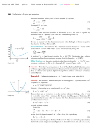
![January 19, 2001 09:46 g65-ch4 Sheet number 57 Page number 297 cyan magenta yellow black
4.6 Applied Maximum and Minimum Problems 297
and ±18. A check of these values shows that x = 2 is a root, so that x − 2 is a factor of the
polynomial. After dividing the polynomial by this factor we can rewrite (22) as
(x − 2)(2x2
+ 4x + 9) = 0
Thus, the remaining solutions of (22) satisfy the quadratic equation
2x2
+ 4x + 9 = 0
But this equation has no real solutions (using the quadratic formula), so that x = 2 is the
only critical number of S. To determine the nature of this critical number we will use the
second derivative test. From (21),
d2
S
dx2
= 12x2
+ 2, so
d2
S
dx2
x=2
= 50 > 0
which shows that a relative minimum occurs at x = 2. Since x = 2 is the only relative
extremum for L, it follows from Theorem 4.5.5 that an absolute minimum value of L also
occurs at x = 2. Thus, the point on the curve y = x2
closest to (18, 0) is
(x, y) = (x, x2
) = (2, 4)
• • • • • • • • • • • • • • • • • • • • • • • • • • • • • • • • • • • • • •
AN APPLICATION TO ECONOMICS
Three functions of importance to an economist or a manufacturer are
C(x) = total cost of producing x units of a product during some time period
R(x) = total revenue from selling x units of the product during the time period
P(x) = total profit obtained by selling x units of the product during the time period
These are called, respectively, the cost function, revenue function, and profit function. If
all units produced are sold, then these are related by
P(x) = R(x) − C(x)
[profit] = [revenue] – [cost]
(23)
The total cost C(x) of producing x units can be expressed as a sum
C(x) = a + M(x) (24)
where a is a constant, called overhead, and M(x) is a function representing manufacturing
cost. The overhead, which includes such fixed costs as rent and insurance, does not depend
on x; it must be paid even if nothing is produced. On the other hand, the manufacturing cost
M(x), which includes such items as cost of materials and labor, depends on the number of
items manufactured. It is shown in economics that with suitable simplifying assumptions,
M(x) can be expressed in the form
M(x) = bx + cx2
where b and c are constants. Substituting this in (24) yields
C(x) = a + bx + cx2
(25)
If a manufacturing firm can sell all the items it produces for p dollars apiece, then its
total revenue R(x) (in dollars) will be
R(x) = px (26)
and its total profit P(x) (in dollars) will be
P(x) = [total revenue] − [total cost] = R(x) − C(x) = px − C(x)
Thus, if the cost function is given by (25),
P(x) = px − (a + bx + cx2
) (27)
Depending on such factors as number of employees, amount of machinery available, eco-
nomic conditions, and competition, there will be some upper limit on the number of items](https://image.slidesharecdn.com/ch04-150306071940-conversion-gate01/85/Ch04-57-320.jpg)
![January 19, 2001 09:46 g65-ch4 Sheet number 58 Page number 298 cyan magenta yellow black
298 The Derivative in Graphing and Applications
a manufacturer is capable of producing and selling. Thus, during a fixed time period the
variable x in (27) will satisfy
0 ≤ x ≤
By determining the value or values of x in [0, ] that maximize (27), the firm can determine
how many units of its product must be manufactured and sold to yield the greatest profit.
This is illustrated in the following numerical example.
Example 7 A liquid form of penicillin manufactured by a pharmaceutical firm is sold in
bulk at a price of $200 per unit. If the total production cost (in dollars) for x units is
C(x) = 500,000 + 80x + 0.003x2
and if the production capacity of the firm is at most 30,000 units in a specified time, how
many units of penicillin must be manufactured and sold in that time to maximize the profit?
Solution. Since the total revenue for selling x units is R(x) = 200x, the profit P (x) on
x units will be
P(x) = R(x) − C(x) = 200x − (500,000 + 80x + 0.003x2
) (28)
Since the production capacity is at most 30,000 units, x must lie in the interval [0, 30,000].
From (28)
dP
dx
= 200 − (80 + 0.006x) = 120 − 0.006x
Setting dP/dx = 0 gives
120 − 0.006x = 0 or x = 20,000
Since this critical number lies in the interval [0, 30,000], the maximum profit must occur
at one of the values
x = 0, x = 20,000, or x = 30,000
Substituting these values in (28) yields Table 4.6.5, which tells us that the maximum profit
P = $700,000 occurs when x = 20,000 units are manufactured and sold in the specified
time.
Table 4.6.5
0
–500,000 700,000
20,000
400,000
30,000x
P(x)
• • • • • • • • • • • • • • • • • • • • • • • • • • • • • • • • • • • • • •
MARGINAL ANALYSIS
Economists call P (x), R (x), and C (x) the marginal profit, marginal revenue, and mar-
ginal cost, respectively; and they interpret these quantities as the additional profit, revenue,
and cost that result from producing and selling one additional unit of the product when
the production and sales levels are at x units. These interpretations follow from the local
linear approximations of the profit, revenue, and cost functions. For example, it follows
from Formula (2) of Section 3.8 that when the production and sales levels are at x units the
local linear approximation of the profit function is
P(x + x) ≈ P(x) + P (x) x
Thus, if x = 1 (one additional unit produced and sold), this formula implies
P(x + 1) ≈ P(x) + P (x)
and hence the additional profit that results from producing and selling one additional unit
can be approximated as
P(x + 1) − P(x) ≈ P (x)](https://image.slidesharecdn.com/ch04-150306071940-conversion-gate01/85/Ch04-58-320.jpg)
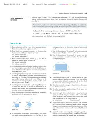
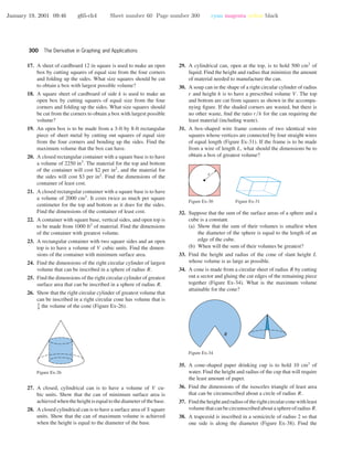
![January 19, 2001 09:46 g65-ch4 Sheet number 61 Page number 301 cyan magenta yellow black
4.6 Applied Maximum and Minimum Problems 301
maximum possible area for the trapezoid. [Hint: Express
the area of the trapezoid in terms of θ.]
39. A drainage channel is to be made so that its cross section
is a trapezoid with equally sloping sides (Figure Ex-39). If
the sides and bottom all have a length of 5 ft, how should
the angle θ (0 ≤ θ ≤ π/2) be chosen to yield the greatest
cross-sectional area of the channel?
u
2
Figure Ex-38
5 ftu
5 ft
Figure Ex-39
40. A lamp is suspended above the center of a round table of ra-
dius r. How high above the table should the lamp be placed
to achieve maximum illumination at the edge of the table?
[Assume that the illumination I is directly proportional to
the cosine of the angle of incidence φ of the light rays and
inversely proportional to the square of the distance l from
the light source (Figure Ex-40).]
41. A plank is used to reach over a fence 8 ft high to support a
wall that is 1 ft behind the fence (Figure Ex-41). What is the
length of the shortest plank that can be used? [Hint: Express
the length of the plank in terms of the angle θ shown in the
figure.]
r
l
Light
source
f
Figure Ex-40
u
1 ft
8 ft
Figure Ex-41
42. A commercial cattle ranch currently allows 20 steers per
acre of grazing land; on the average its steers weigh 2000 lb
at market. Estimates by the Agriculture Department indicate
that the average market weight per steer will be reduced by
50 lb for each additional steer added per acre of grazing
land. How many steers per acre should be allowed in order
for the ranch to get the largest possible total market weight
for its cattle?
43. (a) A chemical manufacturer sells sulfuric acid in bulk at a
price of $100 per unit. If the daily total production cost
in dollars for x units is
C(x) = 100,000 + 50x + 0.0025x2
and if the daily production capacity is at most 7000
units, how many units of sulfuric acid must be manu-
factured and sold daily to maximize the profit?
(b) Would it benefit the manufacturer to expand the daily
production capacity?
(c) Use marginal analysis to approximate the effect on
profit if daily production could be increased from 7000
to 7001 units.
44. A firm determines that x units of its product can be sold
daily at p dollars per unit, where
x = 1000 − p
The cost of producing x units per day is
C(x) = 3000 + 20x
(a) Find the revenue function R(x).
(b) Find the profit function P(x).
(c) Assuming that the production capacity is at most 500
units per day, determine how many units the company
must produce and sell each day to maximize the profit.
(d) Find the maximum profit.
(e) What price per unit must be charged to obtain the
maximum profit?
45. In a certain chemical manufacturing process, the daily
weight y of defective chemical output depends on the total
weight x of all output according to the empirical formula
y = 0.01x + 0.00003x2
where x and y are in pounds. If the profit is $100 per pound
of nondefective chemical produced and the loss is $20 per
pound of defective chemical produced, how many pounds
of chemical should be produced daily to maximize the total
daily profit?
46. The cost c (in dollars per hour) to run an ocean liner at a
constantspeedv (inmilesperhour)isgivenbyc = a + bvn
,
where a, b, and n are positive constants with n > 1. Find
the speed needed to make the cheapest 3000-mi run.
47. Two particles, A and B, are in motion in the xy-plane.
Their coordinates at each instant of time t (t ≥ 0) are given
by xA = t, yA = 2t, xB = 1 − t, and yB = t. Find the
minimum distance between A and B.
48. Follow the directions of Exercise 47, with xA = t, yA = t2
,
xB = 2t, and yB = 2.
49. Prove that (1, 0) is the closest point on the curve x2
+y2
= 1
to (2, 0).
50. Find all points on the curve y =
√
x for 0 ≤ x ≤ 3 that
are closest to, and at the greatest distance from, the point
(2, 0).
51. Find all points on the curve x2
− y2
= 1 closest to (0, 2).
52. Find a point on the curve x = 2y2
closest to (0, 9).](https://image.slidesharecdn.com/ch04-150306071940-conversion-gate01/85/Ch04-61-320.jpg)
![January 19, 2001 09:46 g65-ch4 Sheet number 62 Page number 302 cyan magenta yellow black
302 The Derivative in Graphing and Applications
53. Find the coordinates of the point P on the curve
y =
1
x2
(x > 0)
where the segment of the tangent line at P that is cut off by
the coordinate axes has its shortest length.
54. Find the x-coordinate of the point P on the parabola
y = 1 − x2
(0 < x ≤ 1)
where the triangle that is enclosed by the tangent line at P
and the coordinate axes has the smallest area.
55. Where on the curve y = 1 + x2 −1
does the tangent line
have the greatest slope?
56. A man is floating in a rowboat 1 mile from the (straight)
shoreline of a large lake. A town is located on the shoreline
1 mile from the point on the shoreline closest to the man. As
suggested in the accompanying figure, he intends to row in a
straight line to some point P on the shoreline and then walk
the remaining distance to the town. To what point should
he row in order to reach his destination in the least time if
(a) he can walk 5 mi/h and row 3 mi/h;
(b) he can walk 5 mi/h and row 4 mi/h?
57. A pipe of negligible diameter is to be carried horizontally
around a corner from a hallway 8 ft wide into a hallway 4 ft
wide (Figure Ex-57). What is the maximum length that the
pipe can have? [An interesting discussion of this problem
in the case where the diameter of the pipe is not neglected
is given by Norman Miller in the American Mathematical
Monthly, Vol. 56, 1949, pp. 177–179.]
Rowboat
Town
1 mi
1 mi
Lake
P
Figure Ex-56
8 ft
4 ft
Figure Ex-57
58. If an unknown physical quantity x is measured n times, the
measurements x1, x2, . . . , xn often vary because of uncon-
trollable factors such as temperature, atmospheric pressure,
and so forth. Thus, a scientist is often faced with the prob-
lem of using n different observed measurements to obtain
an estimate ¯x of an unknown quantity x. One method for
making such an estimate is based on the least squares prin-
ciple, which states that the estimate ¯x should be chosen to
minimize
s = (x1 − ¯x)2
+ (x2 − ¯x)2
+ · · · + (xn − ¯x)2
which is the sum of the squares of the deviations between
the estimate ¯x and the measured values. Show that the
estimate resulting from the least squares principle is
¯x =
1
n
(x1 + x2 + · · · + xn)
that is, ¯x is the arithmetic average of the observed values.
59. Suppose that the intensity of a point light source is directly
proportional to the strength of the source and inversely pro-
portional to the square of the distance from the source. Two
point light sources with strengths of S and 8S are separated
by a distance of 90 cm. Where on the line segment between
the two sources is the intensity a minimum?
60. Prove: If f(x) ≥ 0 on an interval I and if f(x) has a
maximum value on I at x0, then f(x) also has a maxi-
mum value at x0. Similarly for minimum values. [Hint: Use
the fact that
√
x is an increasing function on the interval
[0, +ϱ).]
61. Fermat’s (biography on pp. XXX–XXX) principle in optics
states that light traveling from one point to another follows
that path for which the total travel time is minimum. In a uni-
form medium, the paths of “minimum time” and “shortest
distance” turn out to be the same, so that light, if unob-
structed, travels along a straight line. Assume that we have
a light source, a flat mirror, and an observer in a uniform
medium. If a light ray leaves the source, bounces off the mir-
ror, and travels on to the observer, then its path will consist
of two line segments, as shown in Figure Ex-61. According
to Fermat’s principle, the path will be such that the total
travel time t is minimum or, since the medium is uniform,
the path will be such that the total distance traveled from A
to P to B is as small as possible. Assuming the minimum
occurs when dt/dx = 0, show that the light ray will strike
the mirror at the point P where the “angle of incidence” θ1
equals the “angle of reflection” θ2.
a
x
c
b
A
B
P
(Observer)
Mirror
Source
u2 u1
Figure Ex-61
62. Fermat’s principle (Exercise 61) also explains why light
rays traveling between air and water undergo bending (re-
fraction). Imagine that we have two uniform media (such
as air and water) and a light ray traveling from a source
A in one medium to an observer B in the other medium
(Figure Ex-62). It is known that light travels at a constant
speed in a uniform medium, but more slowly in a dense
medium (such as water) than in a thin medium (such as air).
Consequently, the path of shortest time from A to B is not
necessarily a straight line, but rather some broken line path
A to P to B allowing the light to take greatest advantage of](https://image.slidesharecdn.com/ch04-150306071940-conversion-gate01/85/Ch04-62-320.jpg)
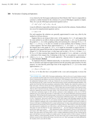
![January 19, 2001 09:46 g65-ch4 Sheet number 65 Page number 305 cyan magenta yellow black
4.7 Newton’s Method 305
x-axis at some point (x2, 0). Substituting the coordinates of this point in (1) yields
−f(x1) = f (x1)(x2 − x1)
Solving for x2 we obtain
x2 = x1 −
f(x1)
f (x1)
(2)
The next approximation can be obtained more easily. If we view x2 as the starting approx-
imation and x3 the new approximation, we can simply apply (2) with x2 in place of x1 and
x3 in place of x2. This yields
x3 = x2 −
f(x2)
f (x2)
(3)
provided f (x2) = 0. In general, if xn is the nth approximation, then it is evident from the
pattern in (2) and (3) that the improved approximation xn+1 is given by
Newton’s Method
xn+1 = xn −
f(xn)
f (xn)
, n = 1, 2, 3, . . .
(4)
Example 1 Use Newton’s Method to approximate the real solutions of
x3
− x − 1 = 0
Solution. Let f(x) = x3
− x − 1, so f (x) = 3x2
− 1 and (4) becomes
xn+1 = xn −
x3
n − xn − 1
3x2
n − 1
(5)
From the graph of f in Figure 4.7.2, we see that the given equation has only one real solu-
tion. This solution lies between 1 and 2 because f(1) = −1 < 0 and f(2) = 5 > 0. We
will use x1 = 1.5 as our first approximation (x1 = 1 or x1 = 2 would also be reasonable
choices).
[–2, 4] × [–3, 3]
xScl = 1, yScl = 1
y = x3
– x – 1
Figure 4.7.2
Letting n = 1 in (5) and substituting x1 = 1.5 yields
x2 = 1.5 −
(1.5)3
− 1.5 − 1
3(1.5)2 − 1
≈ 1.34782609 (6)
(We used a calculator that displays nine digits.) Next, we let n = 2 in (5) and substitute x2
to obtain
x3 = x2 −
x3
2 − x2 − 1
3x2
2 − 1
≈ 1.32520040 (7)
If we continue this process until two identical approximations are generated in succession,
we obtain
x1 ≈ 1.5
x2 ≈ 1.34782609
x3 ≈ 1.32520040
x4 ≈ 1.32471817
x5 ≈ 1.32471796
x6 ≈ 1.32471796
At this stage there is no need to continue further because we have reached the display accu-
racy limit of our calculator, and all subsequent approximations that the calculator generates
will likely be the same. Thus, the solution is approximately x ≈ 1.32471796.](https://image.slidesharecdn.com/ch04-150306071940-conversion-gate01/85/Ch04-65-320.jpg)
![January 19, 2001 09:46 g65-ch4 Sheet number 66 Page number 306 cyan magenta yellow black
306 The Derivative in Graphing and Applications
••
•
•
•
•
•
•
•
•
•
•
•
•
•
•
•
•
•
REMARK. Many calculators and computer programs calculate internally with more digits
than they display. Thus, where possible, you should use stored calculated values rather than
displayed values from intermediate calculations. For example, the value of x2 used in (7)
should be the stored value, not (6).
Example 2 It is evident from Figure 4.7.3 that if x is in radians, then the equation
cos x = x
has a solution between 0 and 1. Use Newton’s Method to approximate it.[0, 5] × [–2, 2]
xScl = 1, yScl = 1
y = cos x
y = x
Figure 4.7.3 Solution. Rewrite the equation as
x − cos x = 0
and apply (4) with f(x) = x − cos x. Since f (x) = 1 + sin x, (4) becomes
xn+1 = xn −
xn − cos xn
1 + sin xn
(8)
From Figure 4.7.3, the solution seems closer to x = 1 than x = 0, so we will use x1 = 1
(radian) as our initial approximation. Letting n = 1 in (8) and substituting x1 = 1 yields
x2 = 1 −
1 − cos 1
1 + sin 1
≈ 0.750363868
Next, letting n = 2 in (8) and substituting this value of x2 yields
x3 = x2
−
x2
− cos x2
1 + sin x2
≈ 0.739112891
If we continue this process until two identical approximations are generated in succession,
we obtain
x1 = 1
x2 ≈ 0.750363868
x3 ≈ 0.739112891
x4 ≈ 0.739085133
x5 ≈ 0.739085133
Thus, to the accuracy limit of our calculator, the solution of the equation cos x = x is
x ≈ 0.739085133.
• • • • • • • • • • • • • • • • • • • • • • • • • • • • • • • • • • • • • •
SOME DIFFICULTIES WITH
NEWTON’S METHOD
When Newton’s Method works, the approximations usually converge toward the solution
with dramatic speed. However, there are situations in which the method fails. For example, if
f (xn) = 0 for some n, then (4) involves a division by zero, making it impossible to generate
xn+1. However, this is to be expected because the tangent line to y = f(x) is parallel to the
x-axis where f (xn) = 0, and hence this tangent line does not cross the x-axis to generate
the next approximation (Figure 4.7.4).
x
y
y = f(x)
f′(x2) = 0
x2 x1
x3 cannot be generated.
Figure 4.7.4
Newton’s Method can fail for other reasons as well; sometimes it may overlook the root
you are trying to find and converge to a different root, and sometimes it may fail to converge
altogether. For example, consider the equation
x1/3
= 0
which has x = 0 as its only solution, and try to approximate this solution by Newton’s
Method with a starting value of x0 = 1. Letting f(x) = x1/3
, Formula (4) becomes
xn+1 = xn −
(xn)1/3
1
3
(xn)−2/3
= xn − 3xn = −2xn
Beginning with x1 = 1, the successive values generated by this formula are
x1 = 1, x2 = −2, x3 = 4, x4 = −8, . . .](https://image.slidesharecdn.com/ch04-150306071940-conversion-gate01/85/Ch04-66-320.jpg)
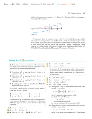
![January 19, 2001 09:46 g65-ch4 Sheet number 68 Page number 308 cyan magenta yellow black
308 The Derivative in Graphing and Applications
makes it possible to perform divisions using multiplications
and subtractions, which is a faster procedure than dividing
directly.
(a) Apply Newton’s Method to
f(x) =
1
x
− a
to derive this approximation.
(b) Use the formula to approximate 1
17
.
21. Use Newton’s Method to find the absolute minimum of
f(x) = 1
4
x4
+ x2
+ 5x
22. Use Newton’s Method to find the absolute maximum of
f(x) = x sin x on the interval [0, π].
23. Use Newton’s Method to find the coordinates of the point
on the parabola y = x2
that is closest to the point (1, 0).
24. Use Newton’s Method to find the dimensions of the rect-
angle of largest area that can be inscribed under the curve
y = cos x for 0 ≤ x ≤ π/2, as shown in the accompanying
figure.
x
y
y = cos x
6
Figure Ex-24
25. (a) Show that on a circle of radius r, the central angle θ that
subtends an arc whose length is 1.5 times the length L
of its chord satisfies the equation θ = 3 sin(θ/2) (see
the accompanying figure).
(b) Use Newton’s Method to approximate θ.
26. A segment of a circle is the region enclosed by an arc and
its chord (see the accompanying figure). If r is the radius
of the circle and θ the angle subtended at the center of the
circle, then it can be shown that the area A of the segment
is A = 1
2
r2
(θ − sin θ), where θ is in radians. Find the value
of θ for which the area of the segment is one-fourth the area
of the circle. Give θ to the nearest degree.
1.5 L
r
u
L
Figure Ex-25
r
u
Figure Ex-26
In Exercises 27 and 28, use Newton’s Method to approxi-
mate all real values of y satisfying the given equation for the
indicated value of x.
27. xy4
+ x3
y = 1; x = 1
28. xy − cos 1
2
xy = 0; x = 2
29. An annuity is a sequence of equal payments that are paid
or received at regular time intervals. For example, you may
want to deposit equal amounts at the end of each year into
an interest-bearing account for the purpose of accumulat-
ing a lump sum at some future time. If, at the end of each
year, interest of i × 100% on the account balance for that
year is added to the account, then the account is said to pay
i × 100% interest, compounded annually. It can be shown
that if payments of Q dollars are deposited at the end of
each year into an account that pays i × 100% compounded
annually, then at the time when the nth payment and the
accrued interest for the past year are deposited, the amount
S(n) in the account is given by the formula
S(n) =
Q
i
[(1 + i)n
− 1]
Suppose that you can invest $5000 in an interest-bearing ac-
count at the end of each year, and your objective is to have
$250,000 on the 25th payment. What annual compound in-
terestratemusttheaccountpayforyoutoachieveyourgoal?
[Hint: Show that the interest rate i satisfies the equation
50i = (1 + i)25
− 1, and solve it using Newton’s Method.]
30. (a) Use a graphing utility to generate the graph of
f(x) =
x
x2 + 1
and use it to explain what happens if you apply New-
ton’s Method with a starting value of x1 = 2. Check
your conclusion by computing x2, x3, x4, and x5.
(b) Use the graph generated in part (a) to explain what hap-
pensifyouapplyNewton’sMethodwithastartingvalue
of x1 = 0.5. Check your conclusion by computing x2,
x3, x4, and x5.
31. (a) Apply Newton’s Method to the function f(x) = x2
+1
with a starting value of x1 = 0.5, and determine if the
values of x2, . . . , x10 appear to converge.
(b) Explain what is happening.](https://image.slidesharecdn.com/ch04-150306071940-conversion-gate01/85/Ch04-68-320.jpg)
![January 19, 2001 09:46 g65-ch4 Sheet number 69 Page number 309 cyan magenta yellow black
4.8 Rolle’s Theorem; Mean-Value Theorem 309
4.8 ROLLE’S THEOREM; MEAN-VALUE THEOREM
In this section we will discuss a result called the Mean-Value Theorem. This theorem
has so many important consequences that it is regarded as one of the major principles
in calculus.
• • • • • • • • • • • • • • • • • • • • • • • • • • • • • • • • • • • • • •
ROLLE’S THEOREM
We will begin with a special case of the Mean-Value Theorem, called Rolle’s Theorem, in
honor of the mathematician Michel Rolle.
∗
This theorem states the geometrically obvious
fact that if the graph of a differentiable function intersects the x-axis at two places, a and
b, then somewhere between a and b there must be at least one place where the tangent line
is horizontal (Figure 4.8.1). The precise statement of the theorem is as follows:
x
a b
y = f(x)
x
a b
y = f(x)
Figure 4.8.1
4.8.1 THEOREM (Rolle’s Theorem). Let f be differentiable on (a, b) and continuous
on [a, b]. If f(a) = f(b) = 0, then there is at least one number c in (a, b) such that
f (c) = 0.
Proof. Either f(x) is equal to zero for all x in [a, b] or it is not. If it is, then f (x) = 0
for all x in (a, b), since f is constant on (a, b). Thus, for any c in (a, b)
f (c) = 0
If f(x) is not equal to zero for all x in [a, b], then there must be a value of x in (a, b) where
f(x) > 0 or f(x) < 0. We will consider the first case and leave the second as an exercise.
Since f is continuous on [a, b], it follows from the Extreme-Value Theorem (4.5.3)
that f has a maximum value at some number c in [a, b]. Since f(a) = f(b) = 0 and
f(x) > 0 somewhere in (a, b), the number c cannot be an endpoint; it must lie in (a, b).
By hypothesis, f is differentiable everywhere on (a, b). In particular, it is differentiable at
c so that f (c) = 0 by Theorem 4.5.4.
Example 1 The function f(x) = sin x has roots at x = 0 and x = 2π. Verify the
hypotheses and conclusion of Rolle’s Theorem for f(x) = sin x on [0, 2π].
Solution. Since f is continuous and differentiable everywhere, it is differentiable on
(0, 2π) and continuous on [0, 2π]. Thus, Rolle’s Theorem guarantees that there is at least
one number c in the interval (0, 2π) such that f (c) = 0. Since f (x) = cos x, we can find
c by solving the equation cos c = 0 on the interval (0, 2π). This yields two values for c,
namely c1 = π/2 and c2 = 3π/2 (Figure 4.8.2).
6 c i o
-1
1
x
y
Figure 4.8.2
∗
MICHEL ROLLE (1652-1719), French mathematician. Rolle, the son of a shopkeeper, received only an elementary
education. He married early and as a young man struggled hard to support his family on the meager wages of
a transcriber for notaries and attorneys. In spite of his financial problems and minimal education, Rolle studied
algebra and Diophantine analysis (a branch of number theory) on his own. Rolle’s fortune changed dramatically in
1682 when he published an elegant solution of a difficult, unsolved problem in Diophantine analysis. The public
recognition of his achievement led to a patronage under minister Louvois, a job as an elementary mathematics
teacher, and eventually to a short-term administrative post in the Ministry of War. In 1685 he joined the Acad´emie
des Sciences in a low-level position for which he received no regular salary until 1699. He stayed there until he
died of apoplexy in 1719.
While Rolle’s fort´e was always Diophantine analysis, his most important work was a book on the algebra
of equations, called Trait´e d’alg`ebre, published in 1690. In that book Rolle firmly established the notation n√
a
[earlier written as n a] for the nth root of a, and proved a polynomial version of the theorem that today bears
his name. (Rolle’s Theorem was named by Giusto Bellavitis in 1846.) Ironically, Rolle was one of the most vocal
early antagonists of calculus. He strove intently to demonstrate that it gave erroneous results and was based on
unsound reasoning. He quarreled so vigorously on the subject that the Acad´emie des Sciences was forced to
intervene on several occasions. Among his several achievements, Rolle helped advance the currently accepted size
order for negative numbers. Descartes, for example, viewed −2 as smaller than −5. Rolle preceded most of his
contemporaries by adopting the current convention in 1691.](https://image.slidesharecdn.com/ch04-150306071940-conversion-gate01/85/Ch04-69-320.jpg)
![January 19, 2001 09:46 g65-ch4 Sheet number 70 Page number 310 cyan magenta yellow black
310 The Derivative in Graphing and Applications
••
•
•
•
•
•
•
•
•
•
•
•
•
•
•
•
•
•
•
•
•
•
•
REMARK. In the preceding example, we were able to find the exact values of c because
the equation f (c) = 0 was easy to solve. However, if this equation cannot be solved, then
you may not be able to find precise values of c, even though you know they exist. This will
rarely cause problems because usually one is more interested in knowing that the values of
c exist than in finding them.
The hypotheses in Rolle’s Theorem are critical—if f fails to be differentiable at even
one place in the interval, then the conclusion may not hold. For example, the function
f(x) = |x| − 1 has roots at x = ±1, yet there is no horizontal tangent line to the graph of
f over the interval (−1, 1) (Figure 4.8.3).
-1 1
-1
1
x
y
y = |x| – 1
Figure 4.8.3
• • • • • • • • • • • • • • • • • • • • • • • • • • • • • • • • • • • • • •
THE MEAN-VALUE THEOREM
Rolle’s Theorem is a special case of the Mean-Value Theorem, which states that between
any two points A and B on the graph of a differentiable function, there must be at least
one place where the tangent line to the curve is parallel to the secant line joining A and B
(Figure 4.8.4).
x
a c b
y = f(x)A(a, f(a))
B(b, f(b))
Figure 4.8.4
Noting that the slope of the secant line joining A(a, f(a)) and B(b, f(b)) is
f(b) − f(a)
b − a
and the slope of the tangent at c is f (c), the Mean-Value Theorem can be stated precisely
as follows.
4.8.2 THEOREM (Mean-Value Theorem). Let f be differentiable on (a, b) and continu-
ous on [a, b]. Then there is at least one number c in (a, b) such that
f (c) =
f(b) − f(a)
b − a
(1)
• • • • • • • • • • • • • • • • • • • • • • • • • • • • • • • • • • • • • •
VELOCITY INTERPRETATION OF
THE MEAN-VALUE THEOREM
There is a nice interpretation of the Mean-Value Theorem in the situation where x = f(t)
is the position versus time curve for a car moving along a straight road. In this case, the
right side of (1) is the average velocity of the car over the time interval from a ≤ t ≤ b,
and the left side is the instantaneous velocity at time t = c. Thus, the Mean-Value Theorem
implies that at least once during the time interval the instantaneous velocity must equal the
average velocity. This agrees with our real-world experience—if the average velocity for a
trip is 40 mi/h, then sometime during the trip the speedometer has to read 40 mi/h.
Example 2 You are driving on a straight highway on which the speed limit is 55 mi/h.
At 8:05 A.M. a police car clocks your velocity at 50 mi/h and at 8:10 A.M. a second police
car posted 5 mi down the road clocks your velocity at 55 mi/h. Explain why the police have
a right to charge you with a speeding violation.
Solution. You traveled 5 mi in 5 min = 1
12
h , so your average velocity was 60 mi/h.
However, the Mean-Value Theorem guarantees the police that your instantaneous velocity
was 60 mi/h at least once over the 5-mi section of highway.
• • • • • • • • • • • • • • • • • • • • • • • • • • • • • • • • • • • • • •
PROOF OF THE MEAN-VALUE
THEOREM
Motivation for the Proof of Theorem 4.8.2. Figure 4.8.4 suggests that (1) will hold
(i.e., the tangent line will be parallel to the secant line) at a number c where the vertical
distance between the curve and the secant line is maximum. Thus, to prove the Mean-Value
Theorem it is natural to begin by looking for a formula for the vertical distance v(x) between
the curve y = f(x) and the secant line joining (a, f(a)) and (b, f(b)).
Proof of Theorem 4.8.2. Since the two-point form of the equation of the secant line
joining (a, f(a)) and (b, f(b)) is
y − f(a) =
f(b) − f(a)
b − a
(x − a)](https://image.slidesharecdn.com/ch04-150306071940-conversion-gate01/85/Ch04-70-320.jpg)
![January 19, 2001 09:46 g65-ch4 Sheet number 71 Page number 311 cyan magenta yellow black
4.8 Rolle’s Theorem; Mean-Value Theorem 311
or equivalently,
y =
f(b) − f(a)
b − a
(x − a) + f(a)
the difference v(x) between the height of the graph of f and the height of the secant line is
v(x) = f(x) −
f(b) − f(a)
b − a
(x − a) + f(a) (2)
Since f(x) is continuous on [a, b] and differentiable on (a, b), so is v(x). Moreover,
v(a) = 0 and v(b) = 0
so that v(x) satisfies the hypotheses of Rolle’s Theorem on the interval [a, b]. Thus, there
is a number c in (a, b) such that v (c) = 0. But from Equation (2)
v (x) = f (x) −
f(b) − f(a)
b − a
so
v (c) = f (c) −
f(b) − f(a)
b − a
Since v (c) = 0, we have
f (c) =
f(b) − f(a)
b − a
Example 3
(a) Generate the graph of f(x) = (x3/4) + 1 over the interval [0, 2], and use it to deter-
mine the number of tangent lines to the graph of f over the interval (0, 2) that are
parallel to the secant line joining the endpoints of the graph.
(b) Show that f satisfies the hypotheses of the Mean-Value Theorem on the interval [0, 2],
and find all values of c in the interval (0, 2) whose existence is guaranteed by the Mean-
ValueTheorem.Confirmthatthesevaluesofc areconsistentwithyourgraphinpart(a).
Solution (a). The graph of f in Figure 4.8.5 suggests that there is only one tangent line
over the interval (0, 2) that is parallel to the secant line joining the endpoints.
Solution (b). The function f is continuous and differentiable everywhere because it is
a polynomial. In particular, f is continuous on [0, 2] and differentiable on (0, 2), so the
hypotheses of the Mean-Value Theorem are satisfied with a = 0 and b = 2. But
f(a) = f(0) = 1, f(b) = f(2) = 3
f (x) =
3x2
4
, f (c) =
3c2
4
so in this case Equation (1) becomes
3c2
4
=
3 − 1
2 − 0
or 3c2
= 4
which has the two solutions c = ±2/
√
3 ≈ ±1.15. However, only the positive solution
lies in the interval (0, 2); this value of c is consistent with Figure 4.8.5.
-2 -1 1 2 3
-1
1
2
3
4
x
y
y = + 1
x3
4
Figure 4.8.5
• • • • • • • • • • • • • • • • • • • • • • • • • • • • • • • • • • • • • •
CONSEQUENCES OF THE
MEAN-VALUE THEOREM
We stated at the beginning of this section that the Mean-Value Theorem is the starting
point for many important results in calculus. As an example of this, we will use it to prove
Theorem 4.1.2, which was one of our fundamental tools for analyzing graphs of functions.](https://image.slidesharecdn.com/ch04-150306071940-conversion-gate01/85/Ch04-71-320.jpg)
![January 19, 2001 09:46 g65-ch4 Sheet number 72 Page number 312 cyan magenta yellow black
312 The Derivative in Graphing and Applications
4.1.2 THEOREM (Revisited). Let f be a function that is continuous on a closed interval
[a, b] and differentiable on the open interval (a, b).
(a) If f (x) > 0 for every value of x in (a, b), then f is increasing on [a, b].
(b) If f (x) < 0 for every value of x in (a, b), then f is decreasing on [a, b].
(c) If f (x) = 0 for every value of x in (a, b), then f is constant on [a, b].
Proof (a). Suppose that x1 and x2 are numbers in [a, b] such that x1 < x2. We must show
that f(x1) < f(x2). Because the hypotheses of the Mean-Value Theorem are satisfied on
the entire interval [a, b], they are satisfied on the subinterval [x1, x2]. Thus, there is some
number c in the open interval (x1, x2) such that
f (c) =
f(x2) − f(x1)
x2 − x1
or equivalently,
f(x2) − f(x1) = f (c)(x2 − x1) (3)
Since c is in the open interval (x1, x2), it follows that a < c < b; thus, f (c) > 0. However,
x2 − x1 > 0 since we assumed that x1 < x2. It follows from (3) that f(x2) − f(x1) > 0 or,
equivalently, f(x1) < f(x2), which is what we were to prove. The proofs of parts (b) and
(c) are similar and are left as exercises.
• • • • • • • • • • • • • • • • • • • • • • • • • • • • • • • • • • • • • •
THE CONSTANT DIFFERENCE
THEOREM
We know from our earliest study of derivatives that the derivative of a constant is zero. Part
(c) of Theorem 4.1.2 is the converse of that result; that is, a function whose derivative is
zero on an interval must be constant on that interval. If we apply this to the difference of
two functions, we obtain the following useful theorem.
4.8.3 THEOREM (The Constant Difference Theorem). If f and g are continuous on a closed
interval [a, b], and if f (x) = g (x) for all x in the open interval (a, b), then f and g
differ by a constant on [a, b]; that is, there is a constant k such that f(x) − g(x) = k
for all x in [a, b].
Proof. Let h(x) = f(x) − g(x). Then for every x in (a, b)
h (x) = f (x) − g (x) = 0
Thus, h(x) = f(x) − g(x) is constant on [a, b] by Theorem 4.1.2(c).
••
•
•
•
•
•
•
•
•
•
•
•
REMARK. This theorem remains true if the closed interval [a, b] is replaced by a finite or
infinite interval (a, b), [a, b), or (a, b], provided f and g are differentiable on (a, b) and
continuous on the entire interval.
The Constant Difference Theorem has a simple geometric interpretation—it tells us that
if f and g have the same derivative on an interval, then there is a constant k such that
f(x) = g(x) + k for each x in the interval; that is, the graphs of f and g can be obtained
from one another by a vertical translation (Figure 4.8.6).
x
y
y = f(x) = g(x) + k
y = g(x)
If f′(x) = g′(x) on an interval,
then the graphs of f and g are
vertical translations of one
another.
k
Figure 4.8.6](https://image.slidesharecdn.com/ch04-150306071940-conversion-gate01/85/Ch04-72-320.jpg)
![January 19, 2001 09:46 g65-ch4 Sheet number 73 Page number 313 cyan magenta yellow black
4.8 Rolle’s Theorem; Mean-Value Theorem 313
EXERCISE SET 4.8 Graphing Calculator
• • • • • • • • • • • • • • • • • • • • • • • • • • • • • • • • • • • • • • • • • • • • • • • • • • • • • • • • • • • • • • • • • • • • • • • • • • • • • • • • • • • • • • • • • • • • • • • • • • • • • • • • • • • • • •
In Exercises 1 and 2, use the graph of f to find an interval
[a, b] on which Rolle’s Theorem applies, and find all values
of c in that interval that satisfy the conclusion of the theorem.
1.
-2 -1 0 1 2 3 4 5
-3
-2
-1
0
1
2
3
x
y
f
2.
–5 –4 –3–2 –1 0 1 2 3 4 5
-7
-6
-5
-4
-3
-2
-1
0
1
2
3
x
y
In Exercises 3–8, verify that the hypotheses of Rolle’s Theo-
rem are satisfied on the given interval, and find all values of
c in that interval that satisfy the conclusion of the theorem.
3. f(x) = x2
− 6x + 8; [2, 4]
4. f(x) = x3
− 3x2
+ 2x; [0, 2]
5. f(x) = cos x; [π/2, 3π/2]
6. f(x) =
x2
− 1
x − 2
; [−1, 1]
7. f(x) = 1
2
x −
√
x; [0, 4]
8. f(x) =
1
x2
−
4
3x
+
1
3
; [1, 3]
9. Use the graph of f in the accompanying figure to estimate
all values of c that satisfy the conclusion of the Mean-Value
Theorem on the interval [0, 8].
0 1 2 3 4 5 6 7 8 9 10
0
1
2
3
4
5
6
7
x
y
Figure Ex-9
10. Use the graph of f in Exercise 9 to estimate all values of c
that satisfy the conclusion of the Mean-Value Theorem on
the interval [0, 4].
In Exercises 11–16, verify that the hypotheses of the Mean-
Value Theorem are satisfied on the given interval, and find
all values of c in that interval that satisfy the conclusion of
the theorem.
11. f(x) = x2
+ x; [−4, 6]
12. f(x) = x3
+ x − 4; [−1, 2]
13. f(x) =
√
x + 1; [0, 3] 14. f(x) = x +
1
x
; [3, 4]
15. f(x) = 25 − x2; [−5, 3]
16. f(x) =
1
x − 1
; [2, 5]
17. (a) Find an interval [a, b] on which
f(x) = x4
+ x3
− x2
+ x − 2
satisfies the hypotheses of Rolle’s Theorem.
(b) Generate the graph of f (x), and use it to make rough
estimates of all values of c in the interval obtained in
part (a) that satisfy the conclusion of Rolle’s Theorem.
(c) Use Newton’s Method to improve on the rough esti-
mates obtained in part (b).
18. Let f(x) = x3
+ 4x.
(a) Find the equation of the secant line through the points
(−2, f(−2)) and (1, f(1)).
(b) Show that there is only one number c in the interval
(−2, 1) that satisfies the conclusion of the Mean-Value
Theorem for the secant line in part (a).
(c) Find the equation of the tangent line to the graph of f
at the point (c, f(c)).
(d) Use a graphing utility to generate the secant line in part
(a) and the tangent line in part (c) in the same coor-
dinate system, and confirm visually that the two lines
seem parallel.
19. Let f(x) = tan x.
(a) Show that there is no number c in the interval (0, π)
such that f (c) = 0, even though f(0) = f(π) = 0.
(b) Explain why the result in part (a) does not violate
Rolle’s Theorem.
20. Let f(x) = x2/3
, a = −1, and b = 8.
(a) Show that there is no number c in (a, b) such that
f (c) =
f(b) − f(a)
b − a
(b) Explain why the result in part (a) does not violate the
Mean-Value Theorem.
21. (a) Show that if f is differentiable on (−ϱ, +ϱ), and if
y = f(x) and y = f (x) are graphed in the same coor-
dinate system, then between any two x-intercepts of f
there is at least one x-intercept of f .
(b) Give some examples that illustrate this.
22. Review Definitions 3.1.3 and 3.1.4 of average and instan-
taneous rate of change of y with respect to x, and use the
Mean-Value Theorem to show that if f is differentiable on
(−ϱ, +ϱ), then for any interval [x0, x1] there is at least one
number in (x0, x1) where the instantaneous rate of change
of y with respect to x is equal to the average rate of change
over the interval.](https://image.slidesharecdn.com/ch04-150306071940-conversion-gate01/85/Ch04-73-320.jpg)
![January 19, 2001 09:46 g65-ch4 Sheet number 74 Page number 314 cyan magenta yellow black
314 The Derivative in Graphing and Applications
In Exercises 23–25, use the result of Exercise 22.
23. An automobile travels 4 mi along a straight road in 5 min.
Show that the speedometer reads exactly 48 mi/h at least
once during the trip.
24. At 11 A.M. on a certain morning the outside temperature
was 76◦
F. At 11 P.M. that evening it had dropped to 52◦
F.
(a) Show that at some instant during this period the tem-
perature was decreasing at the rate of 2◦
F/h.
(b) Suppose that you know that the temperature reached a
high of 88◦
F sometime between 11 A.M. and 11 P.M.
Show that at some instant during this period the tem-
perature was decreasing at a rate greater than 3◦
F/h.
25. Suppose that two runners in a 100-m dash finish in a tie.
Show that they had the same velocity at least once during
the race.
26. Use the fact that
d
dx
(x6
− 2x2
+ x) = 6x5
− 4x + 1
to show that the equation 6x5
− 4x + 1 = 0 has at least one
solution in the interval (0, 1).
27. (a) Use the Constant Difference Theorem (4.8.3) to show
that if f (x) = g (x) for all x in the interval (−ϱ, +ϱ),
and if f and g have the same value at some number x0,
then f(x) = g(x) for all x in (−ϱ, +ϱ).
(b) Use the result in part (a) to confirm the trigonometric
identity sin2
x + cos2
x = 1.
28. (a) Use the Constant Difference Theorem (4.8.3) to show
that if f (x) = g (x) for all x in (−ϱ, +ϱ), and if
f(x0) − g(x0) = c at some number x0, then
f(x) − g(x) = c
for all x in (−ϱ, +ϱ).
(b) Use the result in part (a) to show that the function
h(x) = (x − 1)3
− (x2
+ 3)(x − 3)
is constant for all x in (−ϱ, +ϱ), and find the constant.
(c) Check the result in part (b) by multiplying out and sim-
plifying the formula for h(x).
29. (a) Use the Mean-Value Theorem to show that if f is dif-
ferentiable on an interval I, and if |f (x)| ≤ M for all
values of x in I, then
|f(x) − f(y)| ≤ M|x − y|
for all values of x and y in I.
(b) Use the result in part (a) to show that
|sin x − sin y| ≤ |x − y|
for all real values of x and y.
30. (a) Use the Mean-Value Theorem to show that if f is dif-
ferentiable on an open interval I, and if |f (x)| ≥ M
for all values of x in I, then
|f(x) − f(y)| ≥ M|x − y|
for all values of x and y in I.
(b) Use the result in part (a) to show that
| tan x − tan y| ≥ |x − y|
for all values of x and y in the interval (−π/2, π/2).
(c) Use the result in part (b) to show that
| tan x + tan y| ≥ |x + y|
for all values of x and y in the interval (−π/2, π/2).
31. (a) Use the Mean-Value Theorem to show that
√
y −
√
x <
y − x
2
√
x
if 0 < x < y.
(b) Use the result in part (a) to show that if 0 < x < y,
then
√
xy < 1
2
(x + y).
32. Show that if f is differentiable on an open interval I and
f (x) = 0 on I, the equation f(x) = 0 can have at most
one real root in I.
33. Use the result in Exercise 32 to show the following:
(a) The equation x3
+4x −1 = 0 has exactly one real root.
(b) If b2
− 3ac < 0 and if a = 0, then the equation
ax3
+ bx2
+ cx + d = 0
has exactly one real root.
34. Use the Mean-Value Theorem and the inequality 1
6
√
3 <
0.29 to prove that
1.71 <
√
3 < 1.75
[Hint: Let f(x) =
√
x, a = 3, and b = 4 in the Mean-Value
Theorem.]
35. (a) Show that if f and g are functions for which
f (x) = g(x) and g (x) = −f(x)
for all x, then f 2
(x) + g2
(x) is a constant.
(b) Give an example of functions f and g with this property.
36. Show that if f and g are functions for which
f (x) = g(x) and g (x) = f(x)
for all x, then f 2
(x) − g2
(x) is a constant.
37. Let g(x) = x3
− 4x + 6. Find f(x) so that f (x) = g (x)
and f(1) = 2.
38. Let f and g be continuous on [a, b] and differentiable on
(a, b). Prove: If f(a) = g(a) and f(b) = g(b), then there
is a number c in (a, b) such that f (c) = g (c).
39. Illustrate the result in Exercise 38 by drawing an appropriate
picture.
40. (a) Prove: If f (x) > 0 for all x in (a, b), then f (x) = 0
at most once in (a, b).
(b) Give a geometric interpretation of the result in (a).](https://image.slidesharecdn.com/ch04-150306071940-conversion-gate01/85/Ch04-74-320.jpg)
![January 19, 2001 09:46 g65-ch4 Sheet number 75 Page number 315 cyan magenta yellow black
Supplementary Exercises 315
41. (a) Prove part (b) of Theorem 4.1.2.
(b) Prove part (c) of Theorem 4.1.2.
42. Use the Mean-Value Theorem to prove the following result:
Let f be continuous at x0 and suppose that limx →x0
f (x)
exists. Then f is differentiable at x0, and
f (x0) = lim
x →x0
f (x)
[Hint: The derivative f (x0) is given by
f (x0) = lim
x →x0
f (x) − f (x0)
x − x0
provided this limit exists.]
43. Let
f(x) =
3x2
, x ≤ 1
ax + b, x > 1
Find the values of a and b so that f will be differentiable at
x = 1.
44. (a) Let
f(x) =
x2
, x ≤ 0
x2
+ 1, x > 0
Show that
lim
x →0−
f (x) = lim
x →0+
f (x)
but that f (0) does not exist.
(b) Let
f(x) =
x2
, x ≤ 0
x3
, x > 0
Show that f (0) exists but f (0) does not.
45. Use the Mean-Value Theorem to prove the following result,
alluded to in Section 4.3: The graph of a function f has a
vertical tangent line at (x0, f (x0)) if f is continuous at x0
and f (x) approaches either +ϱ or −ϱ as x → x+
0 and as
x →x−
0 .
SUPPLEMENTARY EXERCISES
Graphing Calculator C CAS
1. (a) If x1 < x2, what relationship must hold between f(x1)
and f(x2) if f is increasing on an interval containing
x1 and x2? Decreasing? Constant?
(b) What condition on f ensures that f is increasing on an
interval [a, b]? Decreasing? Constant?
2. (a) What condition on f ensures that f is concave up on
an open interval I? Concave down?
(b) What condition on f ensures that f is concave up on
an open interval I? Concave down?
(c) In words, what is an inflection point of f ?
3. (a) Where on the graph of y = f(x) would you expect y to
be increasing or decreasing most rapidly with respect
to x?
(b) In words, what is a relative extremum?
(c) State a procedure for determining where the relative
extrema of f occur.
4. Determine whether the statement is true or false. If it is false,
give an example for which the statement fails.
(a) If f has a relative maximum at x0, then f(x0) is the
largest value that f(x) can have.
(b) If f(x0) is the largest value for f on the interval (a, b),
then f has a relative maximum at x0.
(c) A function f has a relative extremum at each of its
critical numbers.
5. (a) According to the first derivative test, what conditions
ensure that f has a relative maximum at x0? A relative
minimum?
(b) According to the second derivative test, what conditions
ensure that f has a relative maximum at x0? A relative
minimum?
6. In each part, sketch a continuous curve y = f(x) with the
stated properties.
(a) f(2) = 4, f (2) = 1, f (x) < 0 for x < 2, f (x) > 0
for x > 2
(b) f(2) = 4, f (x) > 0 for x < 2, f (x) < 0 for x > 2,
and lim
x →2−
f (x) = +ϱ, lim
x →2+
f (x) = +ϱ
(c) f(2) = 4, f (x) < 0 for x = 2, and lim
x →2−
f (x) = 1,
lim
x →2+
f (x) = −1
7. In each part, find all critical numbers, and use the first deriva-
tivetesttoclassifythemasrelativemaxima,relativeminima,
or neither.
(a) f(x) = x1/3
(x − 7)2
(b) f(x) = 2 sin x − cos 2x, 0 ≤ x ≤ 2π
(c) f(x) = 3x − (x − 1)3/2
8. In each part, find all critical numbers, and use the second
derivative test(where possible) to classify them as relative](https://image.slidesharecdn.com/ch04-150306071940-conversion-gate01/85/Ch04-75-320.jpg)
![January 19, 2001 09:46 g65-ch4 Sheet number 76 Page number 316 cyan magenta yellow black
316 The Derivative in Graphing and Applications
maxima, relative minima, or neither.
(a) f(x) = x−1/2
+ 1
9
x1/2
(b) f(x) = x2
+ 8/x
(c) f(x) = sin2
x − cos x, 0 ≤ x ≤ 2π
In Exercises 9–16, give a graph of f , and identify the lim-
its as x → ±ϱ, as well as locations of all relative extrema,
inflection points, and asymptotes (as appropriate).
9. f(x) = x4
− 3x3
+ 3x2
+ 1
10. f(x) = x5
− 4x4
+ 4x3
11. f(x) = tan(x2
+ 1) 12. f(x) = x − cos x
13. f(x) =
x2
x2 + 2x + 5
14. f(x) =
25 − 9x2
x3
15. f(x) =
1
2
x2
, x ≤ 0
−x2
, x > 0
16. f(x) = (1 + x)2/3
(3 − x)1/3
When using a graphing utility, important features of a graph
may be missed if the viewing window is not chosen appro-
priately. This is illustrated in Exercises 17 and 18.
17. (a) Generate the graph of f(x) = 1
3
x3
− 1
400
x over the inter-
val [−5, 5], and make a conjecture about the locations
and nature of all critical numbers.
(b) Find the exact locations of all the critical numbers, and
classify them as relative maxima, relative minima, or
neither.
(c) Confirm the results in part (b) by graphing f over an
appropriate interval.
18. (a) Generate the graph of
f(x) = 1
5
x5
− 7
8
x4
+ 1
3
x3
+ 7
2
x2
− 6x
over the interval [−5, 5], and make a conjecture about
the locations and nature of all critical numbers.
(b) Find the exact locations of all the critical numbers, and
classify them as relative maxima, relative minima, or
neither.
(c) Confirm the results in part (b) by graphing portions of
f over appropriate intervals. [Note: It will not be pos-
sible to find a single window in which all of the critical
numbers are clearly visible.]
19. (a) Use a graphing utility to generate the graphs of y = x
and y = (x3
− 8)/(x2
+ 1) together over the interval
[−5, 5], and make a conjecture about the relationship
between the two graphs.
(b) Use Exercise 48 of Section 4.3 to confirm your conjec-
ture in part (a).
20. In parts (a)–(d), the graph of a polynomial with degree at
most 6 is given. Find equations for polynomials that produce
graphs with these shapes, and check your answers with a
graphing utility.
(a)
-1 1
x
y (b)
-1 1
x
y
(c)
-1 1
x
y (d)
-1 1
x
y
21. Find the equations of the tangent lines at all inflection points
of the graph of
f(x) = x4
− 6x3
+ 12x2
− 8x + 3
22. Use implicit differentiation to show that a function defined
implicitly by sin x+cos y = 2y has a critical number when-
ever cos x = 0. Then use either the first or second derivative
test to classify these critical numbers as relative maxima or
minima.
23. Let
f(x) =
2x3
+ x2
− 15x + 7
(2x − 1)(3x2 + x − 1)
Graph y = f(x), and find the equations of all horizontal
and vertical asymptotes. Explain why there is no vertical
asymptote at x = 1
2
, even though the denominator of f is
zero at that point.
C 24. Let
f(x) =
x5
− x4
− 3x3
+ 2x + 4
x7 − 2x6 − 3x5 + 6x4 + 4x − 8
(a) Use a CAS to factor the numerator and denominator of
f , and use the results to determine the locations of all
vertical asymptotes.
(b) Confirm that your answer is consistent with the graph
of f .
25. For a general quadratic polynomial
f(x) = ax2
+ bx + c (a = 0)
find conditions on a, b, and c to ensure that f is always
increasing or always decreasing on [0, +ϱ).
26. For the general cubic polynomial
f(x) = ax3
+ bx2
+ cx + d (a = 0)
find conditions on a, b, c, and d to ensure that f is always
increasing or always decreasing on (−ϱ, +ϱ).
27. In each part, approximate the coordinates (x, y) of the rel-
ative extrema, and confirm that your answers are consistent
with the graph of f .
(a) f(x) = x2
− sin x](https://image.slidesharecdn.com/ch04-150306071940-conversion-gate01/85/Ch04-76-320.jpg)
![January 19, 2001 09:46 g65-ch4 Sheet number 77 Page number 317 cyan magenta yellow black
Supplementary Exercises 317
(b) f(x) =
√
x4 + 1 −
√
x2 + 1
(c) f(x) =
x
x2 − sin x + 1
28. Approximate to six decimal places the largest value of k
such that the function f(x) = 1 + 2x + x3
− x4
is increas-
ing on (−ϱ, k].
29. (a) Can an object in rectilinear motion reverse direction if
its acceleration is constant? Justify your answer using
a velocity versus time curve.
(b) Can an object in rectilinear motion have increasing
speed and decreasing acceleration? Justify your answer
using a velocity versus time curve.
30. Suppose that the position function of a particle in rectilinear
motion is given by the formula s(t) = t/(t2
+ 5) for t ≥ 0.
(a) Use a graphing utility to generate the position, velocity,
and acceleration versus time curves.
(b) Use the appropriate graph to make a rough estimate of
the time when the particle reverses direction, and then
find that time exactly.
(c) Find the position, velocity, and acceleration at the in-
stant when the particle reverses direction.
(d) Use the appropriate graphs to make rough estimates of
the time intervals on which the particle is speeding up
and the time intervals on which it is slowing down, and
then find those time intervals exactly.
(e) Whendoestheparticlehaveitsmaximumandminimum
velocities?
31. A basketball player, standing near the basket to grab a re-
bound, jumps 76.0 cm vertically.
(a) How much time does the player spend in the top 15.0
cm of the jump and how much time in the bottom 15.0
cm?
(b) In words, explain why basketball players seem to be
suspended in air when they jump.
32. (a) Suppose that an object is released from rest from the
top of a high building. Assuming that a free-fall model
applies and that time is in seconds and distance is in me-
ters, make a table that shows the distance traveled by the
object and its speed to one decimal place at 1-second
increments from t = 0 to t = 4.
(b) Confirm that doubling the elapsed time doubles the ve-
locity, and explain why this happens.
(c) Confirm that doubling the elapsed time increases the
distance traveled by a factor of 4, and explain why this
happens.
C 33. Suppose that the position function of a particle in rectilinear
motion is given by the formula
s(t) =
t2
+ 1
t4 + 1
, t ≥ 0
(a) Use a CAS to find simplified formulas for the velocity
v(t) and the acceleration a(t).
(b) Graph the position, velocity, and acceleration versus
time curves.
(c) Use the appropriate graph to make a rough estimate of
the time at which the particle is farthest from the origin
and its distance from the origin at that time.
(d) Use the appropriate graph to make a rough estimate of
the time interval during which the particle is moving in
the positive direction.
(e) Use the appropriate graphs to make rough estimates of
the time intervals during which the particle is speeding
up and the time intervals during which it is slowing
down.
(f) Use the appropriate graph to make a rough estimate
of the maximum speed of the particle and the time at
which the maximum speed occurs.
34. Is it true or false that a particle in rectilinear motion is speed-
ing up when its velocity is increasing and slowing down
when its velocity is decreasing? Justify your answer.
35. (a) What inequality must f(x) satisfy for the function f to
have an absolute maximum on an interval I at x0?
(b) What inequality must f(x) satisfy for f to have an ab-
solute minimum on I at x0?
(c) What is the difference between an absolute extremum
and a relative extremum?
36. According to the Extreme-Value Theorem, what conditions
on a function f and an interval I guarantee that f will have
both an absolute maximum and an absolute minimum on I?
37. In each part, determine whether the statement is true or false,
and justify your answer.
(a) If f is differentiable on the open interval (a, b), and
if f has an absolute extremum on that interval, then it
must occur at a stationary point of f .
(b) If f is continuous on the open interval (a, b), and if f
has an absolute extremum on that interval, then it must
occur at a stationary point of f .
38. Suppose that f is continuous on the closed interval [a, b]
and differentiable on the open interval (a, b), and suppose
that f(a) = f(b). Is it true or false that f must have at least
one stationary point in (a, b)? Justify your answer.
39. In each part, find the absolute minimum m and the absolute
maximum M of f on the given interval (if they exist), and
state where the absolute extrema occur.
(a) f(x) = 1/x; [−2, −1]
(b) f(x) = x3
− x4
; −1, 3
2
(c) f(x) = x2
(x − 2)1/3
; (0, 3]
40. In each part, find the absolute minimum m and the absolute
maximum M of f on the given interval (if they exist), and
state where the absolute extrema occur.
(a) f(x) = 2x/(x2
+ 3); (0, 2]
(b) f(x) = 2x5
− 5x4
+ 7; (−1, 3)
(c) f(x) = −|x2
− 2x|; [1, 3]
41. Draw an appropriate picture, and describe the basic idea of
Newton’s Method without using any formulas.
42. Use Newton’s Method to approximate all three solutions of
x3
− 4x + 1 = 0.](https://image.slidesharecdn.com/ch04-150306071940-conversion-gate01/85/Ch04-77-320.jpg)
![January 19, 2001 09:46 g65-ch4 Sheet number 78 Page number 318 cyan magenta yellow black
318 The Derivative in Graphing and Applications
43. Use Newton’s Method to approximate the smallest positive
solution of sin x + cos x = 0.
44. Suppose that f is an increasing function on [a, b] and that
x0 is a number in (a, b). Prove that if f is differentiable at
x0, then f (x0) ≥ 0.
45. In each part, determine whether all of the hypotheses of
Rolle’s Theorem are satisfied on the stated interval. If not,
state which hypotheses fail; if so, find all values of c guar-
anteed in the conclusion of the theorem.
(a) f(x) = 4 − x2 on [−2, 2]
(b) f(x) = x2/3
− 1 on [−1, 1]
(c) f(x) = sin(x2
) on [0,
√
π ]
46. In each part, determine whether all of the hypotheses of the
Mean-Value Theorem are satisfied on the stated interval. If
not, state which hypotheses fail; if so, find all values of c
guaranteed in the conclusion of the theorem.
(a) f(x) = |x − 1| on [−2, 2]
(b) f(x) =
x + 1
x − 1
on [2, 3]
(c) f(x) =
3 − x2
if x ≤ 1
2/x if x > 1
on [0, 2]
47. A church window consists of a blue semicircular section
surmounting a clear rectangular section as shown in the ac-
companying figure. The blue glass lets through half as much
light per unit area as the clear glass. Find the radius r of the
window that admits the most light if the perimeter of the
entire window is to be P feet.
48. Find the dimensions of the rectangle of maximum area that
can be inscribed inside the ellipse (x/4)2
+(y/3)2
= 1 (see
the accompanying figure).
Blue
Clear
r
h
Figure Ex-47
(x/4)2
+ (y/3)2
= 1
-4 4
-3
3
x
y
Figure Ex-48
C 49. Let
f(x) =
x3
+ 2
x4 + 1
(a) Generate the graph of y = f(x), and use the graph to
make rough estimates of the coordinates of the absolute
extrema.
(b) Use a CAS to solve the equation f (x) = 0 and then
use it to make more accurate approximations of the co-
ordinates in part (a).
C 50. As shown in the accompanying figure, suppose that a boat
enters the river at the point (1, 0) and maintains a heading
toward the origin. As a result of the strong current, the boat
follows the path
y =
x10/3
− 1
2x2/3
where x and y are in miles.
(a) Graph the path taken by the boat.
(b) Can the boat reach the origin? If not, discuss its fate and
find how close it comes to the origin.
(c) What is the velocity of the boat in the x-direction at the
instant when it is closest to the origin if the velocity in
the y-direction is −4 mi/h at this instant?
(1, 0)
x
y
Figure Ex-50
51. According to Kepler’s law, the planets in our solar system
move in elliptical orbits around the Sun. If a planet’s closest
approach to the Sun occurs at time t = 0, then the distance
r from the center of the planet to the center of the Sun at
some later time t can be determined from the equation
r = a(1 − e cos φ)
where a is the average distance between centers, e is a pos-
itive constant that measures the “flatness” of the elliptical
orbit, and φ is the solution of Kepler’s equation
2πt
T
= φ − e sin φ
in which T is the time it takes for one complete orbit of the
planet. Estimate the distance from the Earth to the Sun when
t = 90 days. [First find φ from Kepler’s equation, and then
use this value of φ to find the distance. Use a = 150 × 106
km, e = 0.0167, and T = 365 days.]
52. Using the formulas in Exercise 51, find the distance from
the planet Mars to the Sun when t = 1 year. For Mars use
a = 228 × 106
km, e = 0.0934, and T = 1.88 years.](https://image.slidesharecdn.com/ch04-150306071940-conversion-gate01/85/Ch04-78-320.jpg)