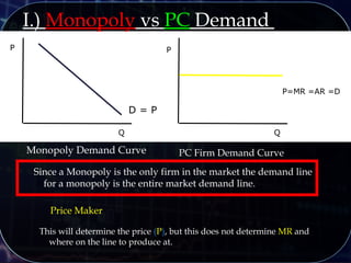
This presentation basically tells how the firm makes decisions in a competitive market. To make concepts here more understable, I have prepared graphs and mathematical equations.
MBA 681 Economics for Strategic DecisionsPrepared by Yun Wan.docxalfredacavx97
MBA 681 Economics for Strategic Decisions
Prepared by Yun Wang
1. How does firm maximize profit.
2. Poduction decision in the perfect competitive market.
3. Production decision in monopolistic competitive market.
4. Production decision in oligopoly.
5. Production decision in monoply.
6. Two special models in oligopoly market.
1. How a Firm Maximizes Profit:
All firms try to maximize profits based on the following equation:
Profit = Total Revenue − Total Cost
The rules we have just developed for profit maximization are:
1. The profit-maximizing level of output is where the difference between total revenue and total
cost is greatest, and
2. The profit-maximizing level of output is also where MR = MC.
Notice: All of these rules do not require the assumption of market type; they are true for all
firms with different market structures (perfect competition, monopolistic competition,
oligopoly, monopoly)!
The Four Market Structures:Structures
Market Structure
Characteristic Perfect Competition
Monopolistic
Competition Oligopoly Monopoly
Type of product Identical Differentiated Identical or differentiated Unique
Ease of entry High High Low Entry blocked
Examples of
industries
Growing wheat
Poultry farming
Clothing stores
Restaurants
Manufacturing computers
Manufacturing automobiles
First-class mail delivery
Providing tap water
2. Profit Determination in Perfect Competitive Market:
A firm maximizes profit at
the level of output at which
marginal revenue equals
marginal cost.
The difference between
price and average total cost
equals profit per unit of
output.
Total profit equals profit per
unit of output, times the
amount of output: the area
of the green rectangle on the
graph.
In the graph on the left, price
never exceeds average cost,
so the firm could not possibly
make a profit.
The best this firm can do is to
break even, obtaining no
profit but incurring no loss.
The MC = MR rule leads us to
this optimal level of
production.
The situation is even worse
for this firm; not only can it
not make a profit, price is
always lower than average
total cost, so it must make
a loss.
It makes the smallest loss
possible by again following
the MC = MR rule.
No other level of output
allows the firm’s loss to be
so small.
Identifying Whether a Firm Can Make a Profit
Once we have determined the quantity where MC = MR, we can immediately know
whether the firm is making a profit, breaking even, or making a loss. At that quantity,
• If P > ATC, the firm is making a profit
• If P = ATC, the firm is breaking even
• If P < ATC, the firm is making a loss
Even better: these statements hold true at every level of output.
However, if the price is too low, i.e. below the minimum point of
AVC, the firm will produce nothing at all.
The quantity supplied is zero below this point.
3. Profit Determination in Monopolistic Competitive Market:
(1 of 3)
In the short run, a monopol.
2024.06.01 Introducing a competency framework for languag learning materials ...Sandy Millin
http://sandymillin.wordpress.com/iateflwebinar2024
Published classroom materials form the basis of syllabuses, drive teacher professional development, and have a potentially huge influence on learners, teachers and education systems. All teachers also create their own materials, whether a few sentences on a blackboard, a highly-structured fully-realised online course, or anything in between. Despite this, the knowledge and skills needed to create effective language learning materials are rarely part of teacher training, and are mostly learnt by trial and error.
Knowledge and skills frameworks, generally called competency frameworks, for ELT teachers, trainers and managers have existed for a few years now. However, until I created one for my MA dissertation, there wasn’t one drawing together what we need to know and do to be able to effectively produce language learning materials.
This webinar will introduce you to my framework, highlighting the key competencies I identified from my research. It will also show how anybody involved in language teaching (any language, not just English!), teacher training, managing schools or developing language learning materials can benefit from using the framework.
Welcome to TechSoup New Member Orientation and Q&A (May 2024).pdfTechSoup
In this webinar you will learn how your organization can access TechSoup's wide variety of product discount and donation programs. From hardware to software, we'll give you a tour of the tools available to help your nonprofit with productivity, collaboration, financial management, donor tracking, security, and more.
June 3, 2024 Anti-Semitism Letter Sent to MIT President Kornbluth and MIT Cor...Levi Shapiro
Letter from the Congress of the United States regarding Anti-Semitism sent June 3rd to MIT President Sally Kornbluth, MIT Corp Chair, Mark Gorenberg
Dear Dr. Kornbluth and Mr. Gorenberg,
The US House of Representatives is deeply concerned by ongoing and pervasive acts of antisemitic
harassment and intimidation at the Massachusetts Institute of Technology (MIT). Failing to act decisively to ensure a safe learning environment for all students would be a grave dereliction of your responsibilities as President of MIT and Chair of the MIT Corporation.
This Congress will not stand idly by and allow an environment hostile to Jewish students to persist. The House believes that your institution is in violation of Title VI of the Civil Rights Act, and the inability or
unwillingness to rectify this violation through action requires accountability.
Postsecondary education is a unique opportunity for students to learn and have their ideas and beliefs challenged. However, universities receiving hundreds of millions of federal funds annually have denied
students that opportunity and have been hijacked to become venues for the promotion of terrorism, antisemitic harassment and intimidation, unlawful encampments, and in some cases, assaults and riots.
The House of Representatives will not countenance the use of federal funds to indoctrinate students into hateful, antisemitic, anti-American supporters of terrorism. Investigations into campus antisemitism by the Committee on Education and the Workforce and the Committee on Ways and Means have been expanded into a Congress-wide probe across all relevant jurisdictions to address this national crisis. The undersigned Committees will conduct oversight into the use of federal funds at MIT and its learning environment under authorities granted to each Committee.
• The Committee on Education and the Workforce has been investigating your institution since December 7, 2023. The Committee has broad jurisdiction over postsecondary education, including its compliance with Title VI of the Civil Rights Act, campus safety concerns over disruptions to the learning environment, and the awarding of federal student aid under the Higher Education Act.
• The Committee on Oversight and Accountability is investigating the sources of funding and other support flowing to groups espousing pro-Hamas propaganda and engaged in antisemitic harassment and intimidation of students. The Committee on Oversight and Accountability is the principal oversight committee of the US House of Representatives and has broad authority to investigate “any matter” at “any time” under House Rule X.
• The Committee on Ways and Means has been investigating several universities since November 15, 2023, when the Committee held a hearing entitled From Ivory Towers to Dark Corners: Investigating the Nexus Between Antisemitism, Tax-Exempt Universities, and Terror Financing. The Committee followed the hearing with letters to those institutions on January 10, 202
Embracing GenAI - A Strategic ImperativePeter Windle
Artificial Intelligence (AI) technologies such as Generative AI, Image Generators and Large Language Models have had a dramatic impact on teaching, learning and assessment over the past 18 months. The most immediate threat AI posed was to Academic Integrity with Higher Education Institutes (HEIs) focusing their efforts on combating the use of GenAI in assessment. Guidelines were developed for staff and students, policies put in place too. Innovative educators have forged paths in the use of Generative AI for teaching, learning and assessments leading to pockets of transformation springing up across HEIs, often with little or no top-down guidance, support or direction.
This Gasta posits a strategic approach to integrating AI into HEIs to prepare staff, students and the curriculum for an evolving world and workplace. We will highlight the advantages of working with these technologies beyond the realm of teaching, learning and assessment by considering prompt engineering skills, industry impact, curriculum changes, and the need for staff upskilling. In contrast, not engaging strategically with Generative AI poses risks, including falling behind peers, missed opportunities and failing to ensure our graduates remain employable. The rapid evolution of AI technologies necessitates a proactive and strategic approach if we are to remain relevant.
Biological screening of herbal drugs: Introduction and Need for
Phyto-Pharmacological Screening, New Strategies for evaluating
Natural Products, In vitro evaluation techniques for Antioxidants, Antimicrobial and Anticancer drugs. In vivo evaluation techniques
for Anti-inflammatory, Antiulcer, Anticancer, Wound healing, Antidiabetic, Hepatoprotective, Cardio protective, Diuretics and
Antifertility, Toxicity studies as per OECD guidelines
Introduction to AI for Nonprofits with Tapp NetworkTechSoup
Dive into the world of AI! Experts Jon Hill and Tareq Monaur will guide you through AI's role in enhancing nonprofit websites and basic marketing strategies, making it easy to understand and apply.
Read| The latest issue of The Challenger is here! We are thrilled to announce that our school paper has qualified for the NATIONAL SCHOOLS PRESS CONFERENCE (NSPC) 2024. Thank you for your unwavering support and trust. Dive into the stories that made us stand out!
Model Attribute Check Company Auto PropertyCeline George
In Odoo, the multi-company feature allows you to manage multiple companies within a single Odoo database instance. Each company can have its own configurations while still sharing common resources such as products, customers, and suppliers.
12. -Three types
Non-Price Discriminating
Price Discriminating
Natural Monopoly
-Then regulating monopolies
Short summary of what we will look at…
IV.) Monopoly
Market Structure
13. Characteristics Perfect
Competition
Monopolistic
Competition
Oligopoly Monopoly
# of sellers Many
(price takers)
Substitution of
Product sold
Only one
product type
from all sellers
Barriers to
entry into
market
No barriers to
enter/ exit
Pricing vs MC
and MR
P =MC=MR
Efficiently Efficient with
zero econ profit
P = AC
One
( no substitutes)
No Substitutes
Almost impossible
for others to
enter market
P > MR
P > MC
P > AC
big LR profits
14. IV.) Monopoly
-only one firm
-Very high barriers to enter market, almost
impossible to start a new business in this market
Price Maker - Can set its own price as high as
customers are willing to pay
15. IV.) Monopoly
Two types of Price Makers to examine side by side
- Charges every customer
the same price.
1.) Non- price
discriminating (normal)
2.) Price discriminating
- If it wants to increase
it’s output it must
decrease the price for
everyone
- Charges every customer
the highest possible price
- Will produce more then
a non-price discriminating
monopoly (normal)
MR ≠ P for this one MR = P for this one
16. (MR) Marginal Revenue
Profit Maximization
∆TR
∆Q
Profit-Maximizing Output: level at which (MR) marginal revenue
equals (MC) marginal cost
MR = MC
We assume all firms are profit maximizing, producing
at the point where their profits are at their highest
(MC) Marginal Cost
∆TC
∆Q
This is still the output answer
but the graph is a little harder
then perfect competition from
before.
17. P
Q
S
D
QQ1
P1
Market D + S
P
PC Firm Demand Curve
P=MR =AR =D
I.) Perfect Competition Demand
This point is a normal profit ( = zero economic profit)
- other firms won’t want to enter the market because there is no
economic (abnormal ) profits
- Output is productively and allocatively efficient
18. P
Q
D = P
Q
Monopoly Demand Curve
P
PC Firm Demand Curve
P=MR =AR =D
I.) Monopoly vs PC Demand
Price Maker
Since a Monopoly is the only firm in the market the demand line
for a monopoly is the entire market demand line.
This will determine the price (P), but this does not determine MR and
where on the line to produce at.
19. IV.) Monopoly Demand
Q
P
****The important thing to understand is that when a monopoly
wants to sell at a larger Q it must lower it’s price on every
single unit made, including ones already made
D = P
To sell a larger Q,
the firm must reduce P
on all units.
Thus, MR ≠ P.
20 40
10
6
20. IV.) Monopoly Demand
Q
P
****The important thing to understand is that when a monopoly
wants to sell at a larger Q it must lower it’s price on every single
unit made, including ones already made
D = P
To sell a larger Q,
the firm must reduce P
on all units.
Thus, MR ≠ P.
20 40
10
6
21. Q P TR AR MR
0 $4.50
1 4.00
2 3.50
3 3.00
4 2.50
5 2.00
6 1.50
n.a.
The table shows the
market demand for
coffee.
Fill in the missing
spaces of the table.
What is the relation
between P and AR?
Between P and MR?
IV.) Monopoly Demand example
22. Here, P = AR,
same as for a
competitive firm.
Here, MR < P,
whereas MR = P
for a competitive
firm.
1.506
2.005
2.504
3.003
3.502
1.50
2.00
2.50
3.00
3.50
$4.004.001
n.a.
9
10
10
9
7
4
$ 0$4.500
MRARTRPQ
–1
0
1
2
3
$4
IV.) Monopoly Demand example
23. Here, P = AR,
same as for a
competitive firm.
Here, MR < P,
whereas MR = P
for a competitive
firm.
1.506
2.005
2.504
3.003
3.502
1.50
2.00
2.50
3.00
3.50
$4.004.001
n.a.
9
10
10
9
7
4
$ 0$4.500
MRARTRPQ
–1
0
1
2
3
$4
IV.) Monopoly Demand example
27. IV.) Monopoly Demand
Q
P
D = P = AR
MR
Profit-Maximizing Q:
Where marginal revenue equals
marginal cost
MR = MC
MC
Step 1
28. IV.) Monopoly Demand
Q
P
D = P = AR
MR
Price:
Profit-Maximizing Q:
Where marginal revenue equals
marginal cost
MR = MC
D = P = AR
Where average revenue
meets the quantity produced
MC
Step 2
29. IV.) Monopoly Demand
Q
P
D = P = AR
To sell a larger Q,
the firm must reduce P
on all units.
Thus, MR ≠ P.
And will always be,
MR < P
MR
Price:
Profit-Maximizing Q:
Where marginal revenue equals
marginal cost
MR = MC
D = P = AR
Where average revenue
meets the quantity produced
MC
ALL old/new
products are at the
new low price
30. Increasing Q has two effects on revenue:
Output effect: higher output raises revenue
Price effect: lower price reduces revenue
To sell a larger Q, the monopolist must reduce the
price on all the units it sells.
Hence, MR < P
MR could even be negative if the price effect exceeds the
output effect
IV.) Monopoly Demand
31. P
Q
D
50
8
B
30
12
A
Demand for coffee
Point A
30 x 12 = 360
Point B
50 x 8 = 400
The total revenue is increased
from 360 to 400. So an increase in
price led to more revenue since
the demand is inelastic, you can
raise your price and make more
money, though less people buy it.
Example Total Revenue Test
Remember the output and
price effect with elasticity?
32. Q
P
D = AR
To sell a larger Q,
the firm must reduce P
on all units.
Thus, MR ≠ P.
And will always be,
MR < P
MR
Price:
P = D = AR
Where average revenue
meets the quantity produced
IV.) Monopoly Demand
34. Q
P
D = AR
MR
MC
Profit-Maximizing Level
Where marginal revenue equals
marginal cost
MR = MC
We assume all firms are profit maximizing, producing
at the point where their profits are at their highest.
IV.) Monopoly Price
Step 1
35. Q
P
D = AR
MR
MC
Profit-Maximizing Level
Where marginal revenue equals
marginal cost
MR = MC
Price:
P = D = AR
Where average revenue
meets the quantity produced
We assume all firms are profit maximizing, producing
at the point where their profits are at their highest.
IV.) Monopoly Price
Step 2
36. Q
P
D = AR
MR
MC
Profit-Maximizing Level
Where marginal revenue equals
marginal cost
MR = MC
Price:
P = D = AR
Where average revenue
meets the quantity produced
We assume all firms are profit maximizing, producing
at the point where their profits are at their highest.
IV.) Monopoly Price
38. Q
P
D = AR
MR
MC
ATC
Q = ATC
Cost:
Profit-Maximizing Level
Where marginal revenue equal
marginal cost
MR = MC
Price:
P = D = AR
Where average revenue
meets the quantity produced
This is a monopoly in the Short
Run and in the Long Run!
IV.) Monopoly Profit
Step 3
39. Q
P
D = AR
MR
MC
ATC
Difference between
AR and ATC
Profit Amount:
Q = ATC
Cost:
Profit-Maximizing Level
Where marginal revenue equal
marginal cost
MR = MC
Price:
P = D = AR
Where average revenue
meets the quantity produced
This is a monopoly in the Short
Run and in the Long Run!
IV.) Monopoly Profit
40. P
Q Q
P
Long RunShort Run
MC
ATC
AR=D
MR
MC
ATC
AR=D
MR
Since there are high barriers to enter the market,
other firms cannot enter the market to change it.
Since a monopoly is the only seller in the market, it
doesn’t have to change and can charge the highest
possible price all the time.
42. Q
P
D
MR
MC
Profit-Maximizing Level
MR = MC
Price
P = D at MR = MC
ATC
Difference between
AR and ATC
Profit Amount
Q = ATC
Cost
IV.) Monopoly Profit
Profit can be a lot
43. Q
P
D
MR
MC
Profit-Maximizing Level
MR = MC
Price
P = D at MR = MC
ATC
Difference between
AR and ATC
Profit Amount
Q = ATC
Cost
IV.) Monopoly Profit
Or a little
44. Q
P
D
MR
MC
Profit-Maximizing Level
MR = MC
Price
P = D at MR = MC
ATC
Difference between
AR and ATC
Profit Amount
Q = ATC
Cost
IV.) Monopoly Profit
Just connect the
dots!
45. P
Q Q
P
Long RunShort Run
MC
ATC
D
MR
MC
ATC
D
MR
Since there are high barriers to enter the market,
other firms cannot enter the market to change it.
Since a monopoly is the only seller in the market, it
doesn’t have to change and can charge the highest
possible price all the time.
47. Q
P
D
MR
MC
ATC
I will remove the ATC curve just to make this easier to read, to find allocative
efficiency since it is not a main curve used to figure out surpluses, just know
that it is there and makes this not all straight lines
Allocative efficiency
Most desirable outcome from
society’s perspective
IV.) Monopoly Welfare Analysis
48. Q
P
D = MB
MR
MC
Monopoly produces at
profit maximizing point
of MR = MC
Allocative efficiency is
MB = MC
So for society we make
MB = D = P = MC
Profit-Maximizing
MR = MC
Surplus-Maximizing
P = MC
IV.) Monopoly Welfare Analysis
These type of monopolies
don’t produce as much as the
market really wants
49. Q
P
D = MB
MR
MC
Monopoly produces at
profit maximizing point
of MR = MC
Allocative efficiency is
MB = MC
So for society we make
MB = D = P = MC
Profit-Maximizing
MR = MC
Surplus-Maximizing
P = MC
IV.) Monopoly Welfare Analysis
They only produce to here
50. Q
P
D = MB
MR
MC
Monopoly produces at
profit maximizing point
of MR = MC
Allocative efficiency is
MB = MC
So for society we make
MB = D = P = MC
Profit-Maximizing
MR = MC
Surplus-Maximizing
P = MC
Deadweight loss to
society
Difference of what production
society wants but Monopoly
actually makes
IV.) Monopoly Welfare Analysis
51. P
Q
S
D
QQ1
P1
Market D + S
P
Perfectly Competitive Firm
MC
MB = MC = max efficient
MC = S
MB = D
ATC
P=MR =AR =D
I.) Perfect Competition Welfare Analysis
MC = S
MB = D = P
P = MC = total
surplus is
maximizedThis is allocative
efficient
53. Q
P
D
MR
MC
Monopoly produces at
profit maximizing point
of MR = MC
Allocative efficiency is
MB = MC
So for society we make
MB = D = P = MC
Profit-Maximizing
MR = MC
Surplus-Maximizing
P = MC
Deadweight loss to
society
Difference of what production
society wants but Monopoly
actually makes
IV.) Monopoly Welfare Analysis
They only produce to here
54. Q
P
D
MR
MC
ATC
For productive efficiency I have to leave in the ATC curve because productive
efficiency is asking if the firm is producing the good or service at the most
efficient point for the firm in regards to society.
Productive efficiency
Producing at the most efficient
possible amount
IV.) Monopoly Welfare Analysis
55. Q
P
D
MR
MC
Monopoly produces at
profit maximizing point
of MR = MC
For society productive
efficiency is Q = min ATC
Profit-Maximizing
MR = MC
Surplus-Maximizing
Q = min ATC
ATC
Monopoly does not do this!
IV.) Monopoly Welfare Analysis
These type of monopolies
don’t produce at the cheapest
point
56. Q
P
D
MR
MC
Monopoly produces at
profit maximizing point
of MR = MC
For society productive
efficiency is Q = min ATC
Profit-Maximizing
MR = MC
Surplus-Maximizing
Q = min ATC
ATC
Monopoly does not do this!
IV.) Monopoly Welfare Analysis
Cost is where ATC = Q
57. Q
P
D
MR
MC
Monopoly produces at
profit maximizing point
of MR = MC
For society productive
efficiency is Q = min ATC
Profit-Maximizing
MR = MC
Surplus-Maximizing
Q = min ATC
Producer surplus
Higher for Monopoly
ATC
Monopoly does not do this!
Consumer surplus
Lower for Consumer
IV.) Monopoly Welfare Analysis
58. Q
P
D
MR
MC
ATC
Abnormal profit - YES
Productively - NO
Efficient
(Q = min ATC )
Allocatively - NO
Efficient ( P = MC )
IV.) Monopoly Welfare Analysis
Monopolies that are profit maximizing are not
producing enough from a society’s perspective
and they are charging too high of a price
59. 歧视 Discrimination: treating people
differently based on some characteristic, e.g.
race or gender.
The characteristic used in price discrimination
is willingness to pay (WTP):
A firm can increase profit by charging a higher
price to buyers with higher WTP.
IV.) Monopoly Power
Price Discrimination: selling the same good
at different prices to different
buyers.
It is sometimes possible for a monopoly to charge
different people difference prices
60. They can charge different prices
and different times when
elasticity is more inelastic like
during Chinese New Year
61. You will pay higher prices for
college then others because of
this price discrimination
62. What makes it possible:
No ability of resale
Lack of information by the
consumer
(asymmetric information)
Income Levels
IV.) Monopoly Power
Price Discrimination: selling the same good
at different prices to different buyers.
Otherwise that means there is no
monopoly of the market
Ignorance of choices though
government ownership,
geographical distance, etc
Richer people tend to have more
inelastic demand so the decision to
buy is less sensitive to price.
63. Willingness to Pay (WTP)
A buyer’s willingness to pay for a good is the
maximum amount the buyer will pay for that good.
WTP measures how much the buyer values the good.
name WTP
Peter 5250
Clara 4500
Wilson 3750
Key 3000
Example:
4 buyers’ WTP
for an iPad
Remember this?
64. WTP and the Demand Curve
At any Q,
the height of
the D curve is
the WTP of the
marginal buyer,
the buyer who
would leave the
market if P were
any higher.
Peters’s WTP
Clara’s WTP
Wilson’s WTP
Key’s WTP
0
750
1500
2250
3000
3750
4500
5250
6000
0 1 2 3 4
P
Q
65. About the Staircase Shape…
If we looked at a larger market with many
more buyers, each would be a step on this
curve
D = MB =P
0
750
1500
2250
3000
3750
4500
5250
6000
0 100200300400500
P
Q
Demand =
Marginal
Benefit
66. IV.) Monopoly Price Discrimination
Q
P
D = AR
MR
MC
ATC
Price discriminating monopoly
charges every single buyer the
highest possible price each will
pay
Profit-Maximizing
D = MC
A price discriminating monopoly will
charge everyone the highest possible
price they can!
4
Peter
Clara
Wilson
Key
321
MR = MC
MR = D
67. IV.) Monopoly Price Discrimination
Q
P
D =MR
MC
ATC
Price discriminating monopoly
charges every single buyer the
highest possible price each will
pay
Profit-Maximizing
MR = D = MC
Producer surplus
Monopoly takes all of it
Consumer surplus
Zero
68. IV.) Monopoly Price Discrimination
Q
P
D =MR
MC
ATC
Price discriminating monopoly
charges every single buyer the
highest possible price each will
pay
Profit-Maximizing
MR = D = MC
Producer surplus
Monopoly takes all of it
Consumer surplus
Zero
But look! These types of
monopolies are allocative
efficient!
69. IV.) Monopoly Power
Is Price Discrimination Bad?
A price discriminating monopoly will charge everyone the
highest possible price they can for each person.
Consumer surplus is zero, and monopolies take all of it.
However because of this they will also produce more output to MC = MB which, from a societies perspective is allocative efficient and everyone that wants
and values the good or service will get it, so there will no longer be a deadweight loss of not enough output.
70. IV.) Monopoly
Two types of Price Makers to examine side by side
- Charges every customer
the same price.
1.) Non- price
discriminating (normal)
2.) Price discriminating
- If it wants to increase
it’s output it must
decrease the price for
everyone
- Charges every customer
the highest possible price
- Will produce more then
a non-price discriminating
monopoly (normal)
MR ≠ P for this one MR = P for this one
71. IV.) Monopoly Welfare Analysis
Q
P
D
MR
MC
Monopoly produces at
profit maximizing point
of MR = MC
Allocative efficiency is
MB = MC
So for society we make
MB = D = P = MC
Profit-Maximizing
MR = MC
Surplus-Maximizing
P = MC
Deadweight loss to society
Difference of what production
society wants but Monopoly
actually makes
Deadweight loss
72. IV.) Monopoly
Two types of Price Makers to examine side by side
- Charges every customer
the same price.
1.) Non- price
discriminating (normal)
2.) Price discriminating
- If it wants to increase
it’s output it must
decrease the price for
everyone
- Charges every customer
the highest possible price
- Will produce more then
a non-price discriminating
monopoly (normal)
MR ≠ P for this one MR = P for this one
73. IV.) Monopoly Price Discrimination
Q
P
D =MR
MC
ATC
Price discriminating monopoly
charges every single buyer the
highest possible price each will
pay
Profit-Maximizing
MR = D = MC
Producer surplus
Monopoly takes all of it
Consumer surplus
Zero
No Deadweight loss!
74. IV.) Monopoly Price Discrimination
Q
P
D =MR
MC
ATC
Abnormal profit - YES
Productively - NO
Efficient
(Q = min ATC )
Allocatively - YES
Efficient ( P = MC )
75. IV.) Monopoly Power
Price Discrimination:
Another way monopolies price discriminate is with Elasticity, but this doesn’t
change the fact that it is an inefficient producer.
76. They charge different people
different prices, but this also
means it can make more money
to have more buses
77. They charge different people
different prices, but this also
means it can make more money
to have more flights
78. P
Q
D
Q
Off peak time
P
Peak demand (Chinese new year)
Another way monopolies price discriminate is with Elasticity.
IV.) Monopoly Price Discrimination
DMR MR
MC
ATC
MC
ATC
They sell the same good or service without any changes to the business itself, but can make an even larger profit due to
increased inelasticity of demand for the good or service
79. Price Discriminating summary:
Monopolies can charge the maximum price that
each different consumer is willing to pay which
also means a monopoly will produce more and
there is no longer a deadweight loss of not
enough output.
Monopolies can also charge a higher price to
everyone based on the elasticity of the demand.
80. Q
P
D
MR
MC
ATC
Abnormal profit - YES
Productively - NO
Efficient
(Q = min ATC )
Allocatively - NO
Efficient ( P = MC )
IV.) Monopoly Welfare Analysis
81. IV.) Monopoly Price Discrimination
Q
P
D =MR
MC
ATC
Abnormal profit - YES
Productively - NO
Efficient
(Q = min ATC )
Allocatively - YES
Efficient ( P = MC )
82. P
Q
D
Q
Off peak time
P
Peak demand (Chinese new year)
Another way monopolies price discriminate is with Elasticity.
IV.) Monopoly Price Discrimination
DMR MR
MC
ATC
MC
ATC
They sell the same good or service without any changes to the business itself, but can make an even larger profit due to
increased inelasticity of demand for the good or service
84. Public goods are in theory unlimited and in making them they
suffer from a problem of how much to make and who pays for
them since everyone gets to enjoy it.
Private
goods
Common
Resource
Natural
Monopolies
Public goods
Excludable Nonexcludable
Rival
Nonrival
IV.) Natural Monopolies
Remember
this?
87. - its use by one person does
not decrease the quantity
available to someone else.
CLASSIFYING GOODS AND RESOURCES
And this?
88. IV.) Natural Monopolies
- It occurs when one large business can supply
the entire market at a lower price than two or
more smaller ones
- A natural monopoly is a situation in which
there cannot be more than one efficient provider
of a good. In this situation, competition might
actually increase costs and prices
- The key point is that a natural monopoly is
characterized by increasing returns to scale at all
levels of output
92. HowHow ATCATC Changes asChanges as
the Scale of Production Changesthe Scale of Production Changes
Economies of scale:
ATC falls
as Q increases.
Constant returns to
scale: ATC stays the
same
as Q increases.
Diseconomies of scale:
ATC rises
as Q increases..
LRATC
Q
ATC
Other typical markets:
93. How ATC Changes as
the Scale of Production Changes
Economies of scale:
ATC falls
as Q increases.
Q
ATC
ATC1
ATC2 ATC3
IV.) Natural Monopolies
The bigger it get the costs
get cheaper at typically
continue to get cheaper
94. -Three types
Non-Price Discriminating
Price Discriminating
Natural Monopoly
-Then regulating monopolies
Short summary of what we will looked at…
IV.) Monopoly
Market Structure
95. P
Q Q
P
Long RunShort Run
MC
ATC
D
MR
MC
ATC
D
MR
Since there are high barriers to enter the market,
other firms cannot enter the market to change it.
Since a monopoly is the only seller in the market, it
doesn’t have to change and can charge the highest
possible price all the time.
96. Q
P
D
MR
MC
ATC
Abnormal profit - YES
Productively - NO
Efficient
(Q = min ATC )
Allocatively - NO
Efficient ( P = MC )
IV.) Monopoly Welfare Analysis
97. P
Q
D
Q
Off peak time
P
Peak demand (Chinese new year)
Another way monopolies price discriminate is with Elasticity.
IV.) Monopoly Price Discrimination
DMR MR
MC
ATC
MC
ATC
They sell the same good or service without any changes to the business itself, but can make an even larger profit due to
increased inelasticity of demand for the good or service
98. IV.) Monopoly Price Discrimination
Q
P
D =MR
MC
ATC
Abnormal profit - YES
Productively - NO
Efficient
(Q = min ATC )
Allocatively - YES
Efficient ( P = MC )
99. IV.) Natural Monopolies
- It occurs when one large business can supply
the entire market at a lower price than two or
more smaller ones
- A natural monopoly is a situation in which
there cannot be more than one efficient provider
of a good. In this situation, competition might
actually increase costs and prices
- The key point is that a natural monopoly is
characterized by increasing returns to scale at all
levels of output
100. Price Discrimination
- Bad for consumers and high prices
Not efficient from a society’s
perspective
- Does not produce as much as people want
Loses the Incentives to Innovate
-Monopoly might not innovate because it doesn’t
have to.
Downsides of a Monopoly
IV.) Monopoly summary
101. Price Discrimination
- Good for Society as more is produced
Capturing Economies of Scale
-Economies of scale can lead to natural monopoly.
-It is more efficient to regulate natural monopoly than to
break it up and make the industry competitive.
Strengthening the Incentives to Innovate
- Monopoly might be more innovative than competition.
-Innovation can create a monopoly.
Benefits of a Monopoly
IV.) Monopoly summary
When the AR column appears, note that AR = P at every quantity. This, of course, is a tautology.
When the MR column appears, note that MR is less than P. This is not as easy to see, because the MR numbers are offset from the rows of the table, just as if you were in an elevator stuck between two floors. But students can still see that MR &lt; P.
For example, in the range of output of Q=2 to Q=3, the price ranges from $3.50 to $3.00, but MR is only $2.
The numbers in the table are from the preceding exercise. Students can see either from the table or the graph that, at any Q, MR &lt; P.
Note that a competitive firm has the output effect but not the price effect: the competitive firm does not need to reduce its price in order to sell a larger quantity, so, for the competitive firm, MR = P.
ing
FYI: The four guys in this example are the members of the Red Hot Chili Peppers. In the corresponding example from the textbook, Mankiw uses the Beatles.
When Q = 1, the height of the demand curve is $300, which is Flea’s willingness to pay, or how much he values an iPod. At any price higher than $300, Flea leaves the market; hence, at Q = 1, Flea is the marginal buyer.
When Q = 2, the height of the demand curve is $250, which is Anthony’s willingness to pay, or how much he values an iPod. At any price higher than $250, Anthony leaves the market; hence, at Q = 2, Anthony is the marginal buyer.
And so forth.
The lesson here is summarized in the text on the right side of the screen: At each Q, the height of the D curve tells you the marginal buyer’s willingness to pay, or how much that buyer values the good.
After the previous slide, most of your students will probably understand where this D curve comes from, but its staircase-like shape will seem quite odd to them.
Point out that it has 4 “steps,” one for each buyer. Suppose there were 10 buyers instead of 4; how many steps would it have? Ten, of course. If there were 20 buyers, this D “curve” would have 20 steps.
A perfectly competitive market has a huge number of buyers. Suppose there were 10,000 buyers in the market for iPods (a tiny fraction of the actual number of buyers!). Then, the number of steps would be 10,000. In relation to the graph, each step would be insignificantly small, and the D curve would look like a smooth curve rather than a staircase – even though it really is a staircase – one with 10,000 infinitesimally small steps.