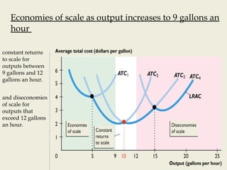
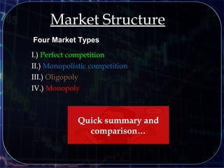
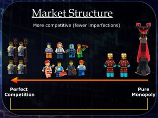
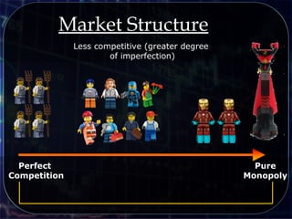
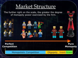
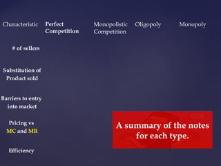
I.) Market structures range from perfect competition to monopoly, with monopolistic competition and oligopoly in between.
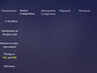
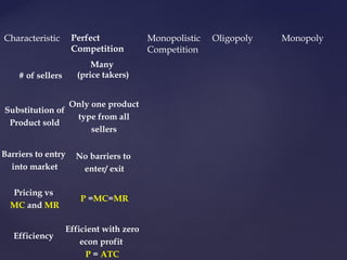
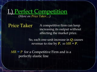
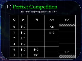
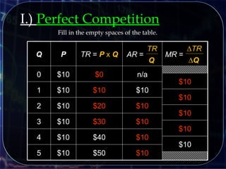
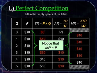
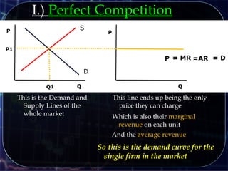
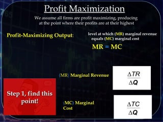
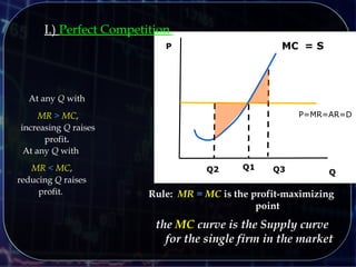
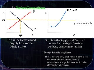
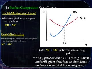
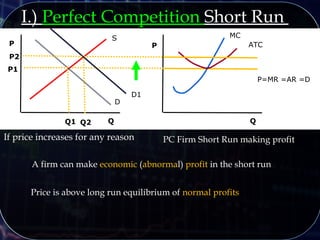
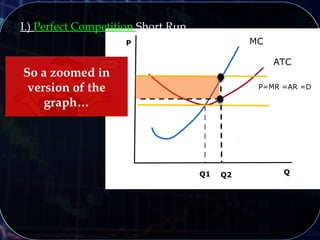
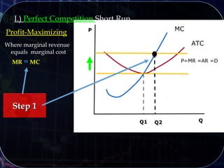
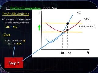
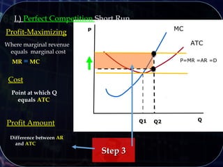
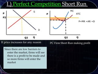
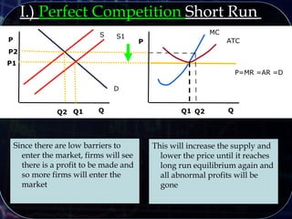
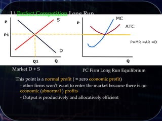
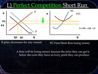
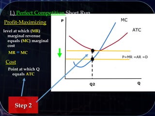
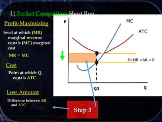
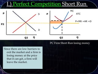
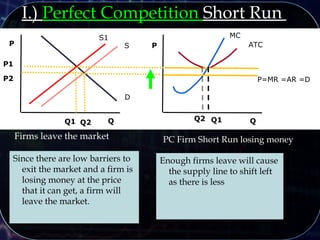
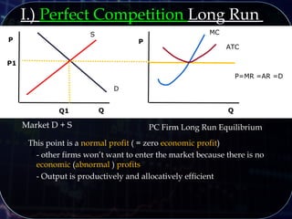
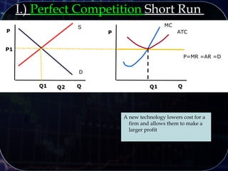
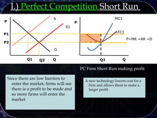
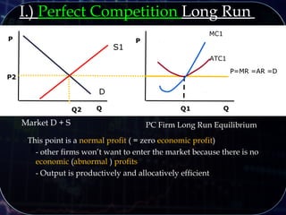
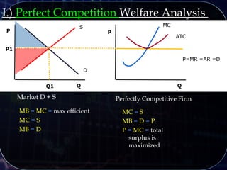
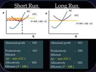
II.) Perfect competition has many small firms, identical products, free entry and exit, and price equal to marginal cost.
III.) Monopoly is the opposite, with a single seller, large barriers to entry, some market control over price, and inefficiency.