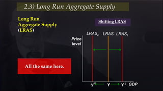
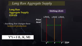
The document discusses the AD/AS model, focusing on long run aggregate supply (LRAS). 1) LRAS is a vertical line, representing the theoretical idea that in the long run, changes in the price level do not affect real output. This comes from classical theories about the separation of nominal and real variables. 2) LRAS can shift due to changes in factors of production like labor, capital, and natural resources. A rightward shift increases potential output while a leftward shift decreases it. 3) Factors that can cause LRAS to shift right include increased investment, population growth, and technological advances, while shifts left can occur due to depleted resources or lower investment.

1. AD/AS Model
(Part 1 – Long Run Supply)

2. AD / AS Model
3.) Short Run Aggregate Supply
1.) Philosophy Bias introduction
2.) Long Run Aggregate Supply
4.) Aggregate Demand
Philosophy part has been removed,
if desired you can download with
the class version PPT.

3. Price
level
GDP
AD
SRAS
PE
LRAS
YN
Graph, trying to explain
the entire economy all
at the same time
Macroeconomics
AD/AS Model

4. Price
level
GDP
PE
LRAS
YN
Graph, trying to explain
the entire economy all
at the same time
Macroeconomics
AD/AS Model
Focus on this curve first, this part
first, might seem like a backwards
way to learn it, but this was the
first curve that was understood
through history.

5. AD / AS Model
3.) Short Run Aggregate Supply
1.) Philosophy Bias introduction
2.) Long Run Aggregate Supply
4.) Aggregate Demand
2.2) LRAS slope
2.3) LRAS shifts
2.1) Classical theory

6. 2.1) Classical Theory
Different parts of this theory that brings us to the conclusions we will work with:
Classical Dichotomy
Quantity Theory of Money
Neutrality of Money
Velocity of Money
- the theoretical 理论 separation of
nominal and real variables.
Hume and the classical economists
suggested that monetary developments
affect nominal variables but not real
variables.

7. all nominal variables –
including prices –
will double.
Nominal variables Real variables
all real variables –
including relative prices –
will remain unchanged.
for example:
If central bank doubles the money supply:
2.1) Classical Theory

8. Gross Domestic Product
(GDP)
国内生产总值
- the total market value of all
goods and services produced
over a specific time period.
- one the primary indicators
used to gauge 测量 the health of
a country's economy.
you can think of it as the
size of the economy.
The same concept of separating
real and nominal variables can also
be seen here.

9. Nominal GDP Real GDP
The Real economy –
Real factors that are independent
of the price level. (actual stuff)
The Money economy –
Measured in the current prices of
output.
2.1) Classical Theory

10. The difference is
that it is adjusting
for inflation.

11. 2.1) Classical Theory
Different parts of this theory that brings us to the conclusions we will work with:
Classical Dichotomy
Quantity Theory of Money
Neutrality of Money
Velocity of Money
(Q of Money) - The quantity of
money determines the
value of money.

12. Marvel
Land
DC
Land
Marvel Land
Money
DC land
Money
(Country B)(Country A)
FOREX graph example
D from B D from A
S from BS from A
So A money =
more valuable
B/A A/B
And B money =
less valuable
Remember this…Remember this?
Value of
money is
based on the
supply and
demand for
the money.

13. 2.1) Classical Theory
Different parts of this theory that brings us to the conclusions we will work with:
Classical Dichotomy
Quantity Theory of Money
Neutrality of Money
Velocity of Money
(N of Money) - In the long run, the overall
price level adjusts to the
level at which the demand
for money equals the
supply of money.
(nominal changes don’t affect real changes)

14. Price
level
GDP
LRAS
Y
P1
P2
2.2) Long Run Aggregate Supply
Long Run
Aggregate Supply
(LRAS)
Change in
money supply
and prices
DON’T change
endowments
能力of factors of
production
Therefore due to
these theories,
prices are
flexible so this
helps explains
why the curve is
vertical.

15. 2.1) Classical Theory
Different parts of this theory that brings us to the conclusions we will work with:
Classical Dichotomy
Quantity Theory of Money
Neutrality of Money
Velocity of Money (V of Money)
Deal with this later when
studying Inflation.

16. AD / AS Model
3.) Short Run Aggregate Supply
1.) Philosophy Bias introduction
2.) Long Run Aggregate Supply
4.) Aggregate Demand
2.2) LRAS slope
2.3) LRAS shifts
2.1) Classical theory

17. 0
1,000
2,000
3,000
4,000
5,000
6,000
0 100 200 300 400 500 600
AxisTitle
Axis Title
The PPC could be a
straight line, or bow-
shaped.
Depends on what
happens to
opportunity cost
as economy shifts
resources from one
industry
to the other.
Production Possibilities Curve
枪炮
黄油
Similar idea as this..
The concept here is
similar, just
instead of trade-
offs of the 2
goods…

18. Price
level
GDP
LRAS
YN
Graph, trying to explain
the entire economy all
at the same time
Macroeconomics
2.) Long Run Aggregate Supply
P1
P2
It’s the trade-off
between the price level
and the whole economy.
The theory is that in
the long run there
really is no trade off, so
it’s a vertical line.

19. Long Run
Aggregate Supply
(LRAS)
- Total average output of an
economy over the long run.
also called
potential output
or
full-employment
output
2.2) Long Run Aggregate Supply
Y*t = f (L, K, M)
Y* is potential output.
t is the time period.
L is the quantity and ability of labor
input available.
K is the available capital stock.
M is the availability of natural
resources.
(factors of production)

20. AD / AS Model
3.) Short Run Aggregate Supply
1.) Philosophy Bias introduction
2.) Long Run Aggregate Supply
4.) Aggregate Demand
2.2) LRAS slope
2.3) LRAS shifts
2.1) classical theory

21. 0
1,000
2,000
3,000
4,000
5,000
6,000
0 100 200 300 400 500 600
AxisTitle
Axis Title
Consumption
goods
Capital
goods
Economic Growth
- Sustained expansion of
the production
possibilities frontier
- to have economic
growth means to
increase the PPF so
more can be produced
without having to
trade-off for as much.
Production Possibilities CurveSimilar idea as this..
Growing this shows
growth...

22. Price
level
GDP
LRAS
Y
LRAS1
Y 1
2.3) Long Run Aggregate Supply
Shifting LRAS
LRAS2
Y
2
Long Run
Aggregate Supply
(LRAS)
The same idea here.

23. Long Run
Aggregate Supply
(LRAS)
2.3) Long Run Aggregate Supply
Y*t = f (L, K, M)
- Anything that changes these
factors of production
Shifting LRAS

24. Long Run
Aggregate Supply
(LRAS)
Shifting LRAS
2.3) Long Run Aggregate Supply
- Changes in L (natural rate of
unemployment)
- Changes in population
examples:
shift right:
- Immigration
- More people get
college degrees
- Lots of older people
retire 退休
- Govt policies reduce
changing job rates
shift left:

25. Long Run
Aggregate Supply
(LRAS)
2.3) Long Run Aggregate Supply
- Changes in K
- Changes in Technology
Shifting LRAS
examples:
- Investment in factories,
equipment
- Productivity improvements
from better technology
- Factories destroyed
by a hurricane飓风
shift left: shift right:

26. Long Run
Aggregate Supply
(LRAS)
2.3) Long Run Aggregate Supply
- Changes in M
- Changes in Natural Resources
Shifting LRAS
examples:
shift left:
- Discovery of new
mineral deposits 矿藏
- Changing weather
patterns that affect farming
- Discovery of new
mineral deposits 矿藏
shift right:

27. To summarize so far…

28. 2.1) Classical Theory
Different parts of this theory that brings us to the conclusions we will work with:
Classical Dichotomy
Quantity Theory of Money
Neutrality of Money
Velocity of Money
(Q of Money)
(N of Money)
(V of Money)

29. Long Run Aggregate Supply
Long Run
Aggregate Supply
(LRAS)
Change in
money supply
and prices
DON’T change
endowments
能力of factors of
production
***Prices are
flexible
Price
level
GDP
LRAS
Y
P1
P2

30. Price
level
GDP
LRAS
Y
LRAS1
Y 1
Long Run Aggregate Supply
Shifting LRAS
LRAS2
Y
2
Y*t = f (L, K, M)
- Anything that changes these
factors of production
Long Run
Aggregate Supply
(LRAS)

31. End of part one. thanks!