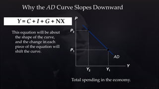
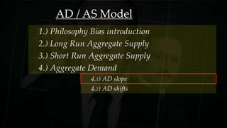
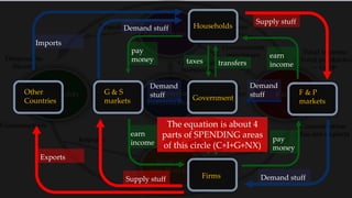
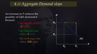
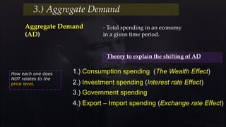
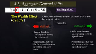
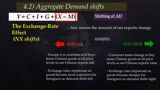
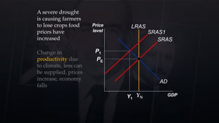
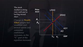
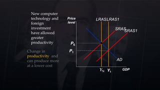
AD/AS Model
(Part 3 – Aggregate Demand)
AD / AS Model
3.) Short Run Aggregate Supply
1.) Philosophy Bias introduction
2.) Long Run Aggregate Supply
4.) Aggregate Demand
P
Y
AD
P1
Y1
P2
Y2 Y1
Y = C + I + G + NX
Aggregate Demand
Total spending in the economy.
This equation will be about
the shape of the curve,
and the change in each
piece of the equation will
shift the curve.
Jean-Baptiste Say (French;
1767 –1832) was a French
economist and businessman. He
had classically liberal views and
argued in favor of competition.
他有古典自由主义的观点,并认为
有利于竞争。
Supply creates it’s
own Demand
Say’s law
Remember this? This helped to
argue that the long run supply
is really important, that
everything goes back to the
long run some how.
John Maynard Keynes, 5 June 1883 – 21 April 1946)
was a British economist whose ideas have fundamentally affected the theory
and practice of modern macroeconomics, and informed the economic
policies of governments. He is widely considered to be one of the founders of
modern macroeconomics and the most influential economist of the 20th
century
Well he said so what?
In the Long Run we are all
dead!!!
Demand creates Supply
Animal spirits 动物精神
消费者信心Consumer
Confidence
Therefore spending now is the key
point that we should focus on.
A great comic that explains
animal spirits…
Time
Short Run
Econ
Growth
Long Run
2.) Business Cycle Model
Peak
Recession
Trough
Expansion
Can see this in the business
cycle.
Also led him to this idea of
the paradox of thrift.
Aggregate Demand
(AD)
3.) Aggregate Demand
- Total spending in an economy
in a given time period.
Y = C + I + G + (X – M)
Y = C + I + G + NX
or
Ceteris Paribus:
• When the P level rises, the Q of real
GDP demanded decreases.
• When the P level falls, the Q of real
GDP demanded increases.
This is the main
equation of
macroeconomics!!!
Why the AD Curve Slopes Downward
P
Y
AD
P1
Y1
P2
Y2 Y1
Y = C + I + G + NX
This equation will be about
the shape of the curve,
and the change in each
piece of the equation will
shift the curve.
Total spending in the economy.
AD / AS Model
3.) Short Run Aggregate Supply
1.) Philosophy Bias introduction
2.) Long Run Aggregate Supply
4.) Aggregate Demand
4.1) AD slope
4.2) AD shifts
Why the AD Curve Slopes Downward?
Assume G fixed
by govt policy.
To understand
the slope of AD,
must determine
how a change in P affects C, I, and NX.
P
Y
AD
P1
Y1
P2
Y2 Y1
4.1) Aggregate Demand slope
G will be discussed
later, so ignore G for
now.
Aggregate Demand
(AD)
4.) Aggregate Demand
1.) Consumption spending (The Wealth Effect)
3.) Government spending
4.) Export – Import spending (Exchange rate Effect)
2.) Investment spending (Interest rate Effect)
Theory to explain slope of AD
- Total spending in an economy
in a given time period.
How each one relates
to the price level.
Households
Firms
G & S
markets
Demand stuff
Supply stuff
pay
money
earn
income
F & P
markets
Demand stuff
Supply stuff
earn
income
pay
money
Government
transferstaxes
taxessubsidies
Demand
stuff
Demand
stuffOther
Countries
Imports
Exports
The equation is about 4
parts of SPENDING areas
of this circle (C+I+G+NX)
Y = C + I + G + (X – M)
C = consumption – of G&S in an economy.
It is typically the largest part of
an economy.
4.1) Aggregate Demand slope
Y = C + I + G + (X – M)
4.1) Aggregate Demand slope
- Change in purchasing powerThe Wealth Effect
(P and C )
Suppose P rises.
- The dollars people hold buy
fewer G&S, so real wealth is lower.
- People feel poorer.
Result: C falls.
example:
Y = C + I + G + (X – M)
C = consumption
4.1) Aggregate Demand slope
I = investment – spending of capital in an economy.
Not stocks and bonds!
Y = C + I + G + (X – M)
4.1) Aggregate Demand slope
- Change in desire to investThe Interest-Rate
Effect
(P and I )
Suppose P rises.
-Buying G&S requires more dollars.
- People demand use of more dollars which
drives up interest rates.
- Higher interest rates mean less investment.
Result: I falls.
example:
Y = C + I + G + (X – M)
C = consumption
4.1) Aggregate Demand slope
I = investment
G = government spending – net after taxes.
Now = Ceteris Paribus,
governments try to control the
economy, a topic for later
Y = C + I + G + (X – M)
C = consumption
4.1) Aggregate Demand slope
I = investment
G = government spending
X-M = exports - imports – net exports.
NX
Y = C + I + G + (X – M)
4.1) Aggregate Demand slope
- Booms/recessions in countries
change export and importing
rates.
- Appreciation/depreciation change
export and importing rates.
- Changes of value of money on
FOREX change imports and exports.
The Exchange-Rate
Effect
(P and NX )
Y = C + I + G + (X – M)
4.1) Aggregate Demand slope
- Changes of value of money on
FOREX change imports and exports.
The Exchange-Rate
Effect
(P and NX ) example:
Suppose P rises.
- U.S. interest rates rise (the interest-rate effect).
- Foreign investors desire more U.S. bonds.
-Higher demand for $ in foreign exchange market.
- U.S. exchange rate appreciates.
- U.S. exports more expensive to people abroad,
imports cheaper to U.S. residents.
Result: NX falls.
An increase in P reduces the
quantity of G&S demanded
because:
P
Y
AD
P1
Y1
 the wealth effect
(C falls)
P2
Y2
 the interest-rate
effect (I falls)
 the exchange-rate
effect (NX falls)
4.1) Aggregate Demand slope
AD / AS Model
3.) Short Run Aggregate Supply
1.) Philosophy Bias introduction
2.) Long Run Aggregate Supply
4.) Aggregate Demand
4.1) AD slope
4.2) AD shifts
Aggregate Demand
(AD)
3.) Aggregate Demand
1.) Consumption spending (The Wealth Effect)
3.) Government spending
4.) Export – Import spending (Exchange rate Effect)
2.) Investment spending (Interest rate Effect)
Theory to explain the shifting of AD
- Total spending in an economy
in a given time period.
How each one does
NOT relates to the
price level.
Any event that changes C, I, G, or NX
– That is NOT a change in P –
will shift the AD curve.
example:
A stock market boom makes
households feel wealthier, C rises,
the AD curve shifts right.
P
Y
AD1
AD2
Y2
P1
Y1
4.2) Aggregate Demand shifts
- Any reason consumption changes that is not
because of price.
- People decide to
saving more money
for retirement.
examples:
shift left: shift right:
- A decrease in taxes
encourages people to
spend more.
4.2) Aggregate Demand shifts
Y = C + I + G + (X – M)
The Wealth Effect
(C shifts )
- People feel good about
the future and increase
spending today.
- People feel bad about
the future and decrease
spending and save
more.
Shifting of AD
The Interest-Rate
Effect (I shifts)
- Firms are unsure about
future business conditions
and cut back on investment
spending.
- Increase in taxes on
business, lowers
investment spending.
- Any reason investment changes that is not
because of price, a change in investor confidence.
- Companies invest in new
computers increases
demand for them.
- A decrease in interest rates
leads to more investment
spending.
4.2) Aggregate Demand shifts
Y = C + I + G + (X – M)
examples:
shift left: shift right:
Shifting of AD
4.2) Aggregate Demand shifts
Y = C + I + G + (X – M)
examples:
shift left: shift right:
- Government decisions that change the overall
economy.
Government spending
- Government buys a new
weapon system.
- Government builds more
highways.
- Government spends less
money on infrastructure.
- Government collects less
taxes and spends less on
public goods.
Shifting of AD
4.2) Aggregate Demand shifts
Y = C + I + G + (X – M)
examples:
shift left: shift right:
The Exchange-Rate
Effect
(NX shifts)
- Any reason the amount of net exports change.
- Europe is in recession so it buys
fewer Chinese goods at all price
levels so net Chinese exports fall.
- Exchange rates Appreciate so
goods become more expensive for
foreigners so demand shifts left.
- Consumer tastes change to buy
more Chinese goods at all price
levels so net Chinese exports raise.
- Exchange rates depreciate so
goods become cheaper for
foreigners so demand shifts right.
Shifting of AD
To summarize it all…
Jean-Baptiste Say (French;
1767 –1832) was a French
economist and businessman. He
had classically liberal views and
argued in favor of competition.
他有古典自由主义的观点,并认为
有利于竞争。
Supply creates it’s
own Demand
Say’s law
2.1) Classical Theory
Different parts of this theory that brings us to the conclusions we will work with:
Classical Dichotomy
Quantity Theory of Money
Neutrality of Money
Velocity of Money
(Q of Money)
(N of Money)
(V of Money)
Long Run Aggregate Supply
Long Run
Aggregate Supply
(LRAS)
***Prices are
flexible
Price
level
GDP
LRAS
Y
P1
P2
An increase in P
does not affect
any of these,
so it does not
affect Y
(Classical dichotomy)
Price
level
GDP
LRAS
Y
LRAS1
Y 1
Long Run Aggregate Supply
Shifting LRAS
LRAS2
Y
2
Y*t = f (L, K, M)
- Anything that changes these
factors of production
Long Run
Aggregate Supply
(LRAS)
John Maynard Keynes, 5 June 1883 – 21 April 1946)
was a British economist whose ideas have fundamentally affected the theory
and practice of modern macroeconomics, and informed the economic
policies of governments. He is widely considered to be one of the founders of
modern macroeconomics and the most influential economist of the 20th
century
In the Long Run
we are all dead!!!!
Price
level
GDP
LRAS
Y
SRAS
Aggregate Supply
is:
 vertical in
long run
 upward-sloping
in short run
AD/AS Model
P
Y
SRAS
Y2
P1
Y1
P2
upward sloping because:
- Over the period
of 1-2 years,
an increase in prices
(P) causes an increase
in the quantity (Y) of
G & S supplied.
Short Run
Aggregate Supply
(SRAS)
3.) Short Run Aggregate Supply
Short Run
Aggregate Supply
(SRAS)
3.2) Short Run Aggregate Supply
- Upward supply curve of the
macro economy that responds
to prices in the short run.
1.) Resource prices are sticky
3.) Change in output costs
4.) Misperceptions
2.) Price changes can be sticky
Theories to explain slope of SRAS
In each there is some type
of market imperfection
Demand creates Supply
Animal spirits
动物精神
消费者信心Consumer Confidence
Why the AD Curve Slopes Downward?
Assume G fixed
by govt policy.
To understand
the slope of AD,
must determine
how a change in P affects C, I, and NX.
P
Y
AD
P1
Y1
P2
Y2 Y1
4.1) Aggregate Demand slope
Aggregate Demand
(AD)
4.) Aggregate Demand
1.) Consumption spending (The Wealth Effect)
3.) Government spending
4.) Export – Import spending (Exchange rate Effect)
2.) Investment spending (Interest rate Effect)
Theory to explain slope of AD
- Total spending in an economy
in a given time period.
How each one relates
to the price level.
Any event that changes C, I, G, or NX
– That is NOT a change in P –
will shift the AD curve.
example:
A stock market boom makes
households feel wealthier, C rises,
the AD curve shifts right.
P
Y
AD1
AD2
Y2
P1
Y1
4.2) Aggregate Demand shifts
Aggregate Demand
(AD)
3.) Aggregate Demand
1.) Consumption spending (The Wealth Effect)
3.) Government spending
4.) Export – Import spending (Exchange rate Effect)
2.) Investment spending (Interest rate Effect)
Theory to explain the shifting of AD
- Total spending in an economy
in a given time period.
How each one does
NOT relates to the
price level.
A few examples to help…
Decide whether an
event shifts LRAS, SRAS
or AD
Price
level
GDP
AD
SRAS
PE
LRAS
YN
A severe drought
is causing farmers
to lose crops food
prices have
increased
SRAS1
Y1
P1Change in
productivity due
to climate, less can
be supplied, prices
increase, economy
falls
Price
level
GDP
AD
SRAS
PE
LRAS
YN Y1
There is a
sustained mass
immigration移民
into the country
LRAS1
SRAS1
AD1
Change in L factor
of production, so
changes long and
size of the
economy to higher
output, regardless
of prices in the
long run
Price
level
GDP
AD
SRAS
PE
LRAS
YN
SRAS1
Y1
P1
Nominal
wages
have
increased
Change in
productivity due
to higher costs to
produce things,
therefore higher
prices and less
output
Price
level
GDP
AD
SRAS
PE
LRAS
YN Y1
P1
The stock
market is doing
very well and is
having record
days
AD1
Change in Wealth
Effect people feel
wealthier and
animal spirits and
consumer
confidence
increases, so the
“C” part of the
equation increases
Price
level
GDP
AD
SRAS
PE
LRAS
YN Y1
P1
AD1
Currency
depreciates
Change in Forex
effect prices seem
cheaper for
foreigners
therefore increased
exports, so the
“NX” part of the
equation increases
Price
level
GDP
AD
SRAS
PE
LRAS
YN
SRAS1
Y1
P1
Government
decides to
raise taxes
Change in taxes,
costs to produce
are higher
therefore prices in
the market are
higher and less
output
Price
level
GDP
AD
SRAS
PE
LRAS
YN Y1
P1
AD1
Government
decides to cut
interest rates
for the central
bank
Change in interest
rate effect it’s cheaper
to borrow so
investment spending
increases, so the “I”
part of the equation
has increased
Price
level
GDP
AD
SRAS
PE
LRAS
YN Y1
LRAS1
SRAS1
New computer
technology and
foreign
investment
have allowed
greater
productivity
P1Change in
productivity and
can produce more
at a lower cost
Price
level
GDP
AD
SRAS
PE
LRAS
YN Y1
P1
AD1
The government
has decided to
spend 4 trillion
Yuan to build
bridges and new
trains
Change in
government
spending so the
“G” part of the
equation has
increased
The End
Thanks


AD SFLS

  • 1.
    AD/AS Model (Part 3– Aggregate Demand)
  • 2.
    AD / ASModel 3.) Short Run Aggregate Supply 1.) Philosophy Bias introduction 2.) Long Run Aggregate Supply 4.) Aggregate Demand
  • 3.
    P Y AD P1 Y1 P2 Y2 Y1 Y =C + I + G + NX Aggregate Demand Total spending in the economy. This equation will be about the shape of the curve, and the change in each piece of the equation will shift the curve.
  • 4.
    Jean-Baptiste Say (French; 1767–1832) was a French economist and businessman. He had classically liberal views and argued in favor of competition. 他有古典自由主义的观点,并认为 有利于竞争。 Supply creates it’s own Demand Say’s law Remember this? This helped to argue that the long run supply is really important, that everything goes back to the long run some how.
  • 5.
    John Maynard Keynes,5 June 1883 – 21 April 1946) was a British economist whose ideas have fundamentally affected the theory and practice of modern macroeconomics, and informed the economic policies of governments. He is widely considered to be one of the founders of modern macroeconomics and the most influential economist of the 20th century Well he said so what? In the Long Run we are all dead!!!
  • 6.
  • 7.
    Animal spirits 动物精神 消费者信心Consumer Confidence Thereforespending now is the key point that we should focus on.
  • 8.
    A great comicthat explains animal spirits…
  • 9.
    Time Short Run Econ Growth Long Run 2.)Business Cycle Model Peak Recession Trough Expansion Can see this in the business cycle.
  • 10.
    Also led himto this idea of the paradox of thrift.
  • 11.
    Aggregate Demand (AD) 3.) AggregateDemand - Total spending in an economy in a given time period. Y = C + I + G + (X – M) Y = C + I + G + NX or Ceteris Paribus: • When the P level rises, the Q of real GDP demanded decreases. • When the P level falls, the Q of real GDP demanded increases. This is the main equation of macroeconomics!!!
  • 12.
    Why the ADCurve Slopes Downward P Y AD P1 Y1 P2 Y2 Y1 Y = C + I + G + NX This equation will be about the shape of the curve, and the change in each piece of the equation will shift the curve. Total spending in the economy.
  • 13.
    AD / ASModel 3.) Short Run Aggregate Supply 1.) Philosophy Bias introduction 2.) Long Run Aggregate Supply 4.) Aggregate Demand 4.1) AD slope 4.2) AD shifts
  • 14.
    Why the ADCurve Slopes Downward? Assume G fixed by govt policy. To understand the slope of AD, must determine how a change in P affects C, I, and NX. P Y AD P1 Y1 P2 Y2 Y1 4.1) Aggregate Demand slope G will be discussed later, so ignore G for now.
  • 15.
    Aggregate Demand (AD) 4.) AggregateDemand 1.) Consumption spending (The Wealth Effect) 3.) Government spending 4.) Export – Import spending (Exchange rate Effect) 2.) Investment spending (Interest rate Effect) Theory to explain slope of AD - Total spending in an economy in a given time period. How each one relates to the price level.
  • 16.
    Households Firms G & S markets Demandstuff Supply stuff pay money earn income F & P markets Demand stuff Supply stuff earn income pay money Government transferstaxes taxessubsidies Demand stuff Demand stuffOther Countries Imports Exports The equation is about 4 parts of SPENDING areas of this circle (C+I+G+NX)
  • 17.
    Y = C+ I + G + (X – M) C = consumption – of G&S in an economy. It is typically the largest part of an economy. 4.1) Aggregate Demand slope
  • 18.
    Y = C+ I + G + (X – M) 4.1) Aggregate Demand slope - Change in purchasing powerThe Wealth Effect (P and C ) Suppose P rises. - The dollars people hold buy fewer G&S, so real wealth is lower. - People feel poorer. Result: C falls. example:
  • 19.
    Y = C+ I + G + (X – M) C = consumption 4.1) Aggregate Demand slope I = investment – spending of capital in an economy. Not stocks and bonds!
  • 20.
    Y = C+ I + G + (X – M) 4.1) Aggregate Demand slope - Change in desire to investThe Interest-Rate Effect (P and I ) Suppose P rises. -Buying G&S requires more dollars. - People demand use of more dollars which drives up interest rates. - Higher interest rates mean less investment. Result: I falls. example:
  • 21.
    Y = C+ I + G + (X – M) C = consumption 4.1) Aggregate Demand slope I = investment G = government spending – net after taxes. Now = Ceteris Paribus, governments try to control the economy, a topic for later
  • 22.
    Y = C+ I + G + (X – M) C = consumption 4.1) Aggregate Demand slope I = investment G = government spending X-M = exports - imports – net exports. NX
  • 23.
    Y = C+ I + G + (X – M) 4.1) Aggregate Demand slope - Booms/recessions in countries change export and importing rates. - Appreciation/depreciation change export and importing rates. - Changes of value of money on FOREX change imports and exports. The Exchange-Rate Effect (P and NX )
  • 24.
    Y = C+ I + G + (X – M) 4.1) Aggregate Demand slope - Changes of value of money on FOREX change imports and exports. The Exchange-Rate Effect (P and NX ) example: Suppose P rises. - U.S. interest rates rise (the interest-rate effect). - Foreign investors desire more U.S. bonds. -Higher demand for $ in foreign exchange market. - U.S. exchange rate appreciates. - U.S. exports more expensive to people abroad, imports cheaper to U.S. residents. Result: NX falls.
  • 25.
    An increase inP reduces the quantity of G&S demanded because: P Y AD P1 Y1  the wealth effect (C falls) P2 Y2  the interest-rate effect (I falls)  the exchange-rate effect (NX falls) 4.1) Aggregate Demand slope
  • 26.
    AD / ASModel 3.) Short Run Aggregate Supply 1.) Philosophy Bias introduction 2.) Long Run Aggregate Supply 4.) Aggregate Demand 4.1) AD slope 4.2) AD shifts
  • 27.
    Aggregate Demand (AD) 3.) AggregateDemand 1.) Consumption spending (The Wealth Effect) 3.) Government spending 4.) Export – Import spending (Exchange rate Effect) 2.) Investment spending (Interest rate Effect) Theory to explain the shifting of AD - Total spending in an economy in a given time period. How each one does NOT relates to the price level.
  • 28.
    Any event thatchanges C, I, G, or NX – That is NOT a change in P – will shift the AD curve. example: A stock market boom makes households feel wealthier, C rises, the AD curve shifts right. P Y AD1 AD2 Y2 P1 Y1 4.2) Aggregate Demand shifts
  • 29.
    - Any reasonconsumption changes that is not because of price. - People decide to saving more money for retirement. examples: shift left: shift right: - A decrease in taxes encourages people to spend more. 4.2) Aggregate Demand shifts Y = C + I + G + (X – M) The Wealth Effect (C shifts ) - People feel good about the future and increase spending today. - People feel bad about the future and decrease spending and save more. Shifting of AD
  • 30.
    The Interest-Rate Effect (Ishifts) - Firms are unsure about future business conditions and cut back on investment spending. - Increase in taxes on business, lowers investment spending. - Any reason investment changes that is not because of price, a change in investor confidence. - Companies invest in new computers increases demand for them. - A decrease in interest rates leads to more investment spending. 4.2) Aggregate Demand shifts Y = C + I + G + (X – M) examples: shift left: shift right: Shifting of AD
  • 31.
    4.2) Aggregate Demandshifts Y = C + I + G + (X – M) examples: shift left: shift right: - Government decisions that change the overall economy. Government spending - Government buys a new weapon system. - Government builds more highways. - Government spends less money on infrastructure. - Government collects less taxes and spends less on public goods. Shifting of AD
  • 32.
    4.2) Aggregate Demandshifts Y = C + I + G + (X – M) examples: shift left: shift right: The Exchange-Rate Effect (NX shifts) - Any reason the amount of net exports change. - Europe is in recession so it buys fewer Chinese goods at all price levels so net Chinese exports fall. - Exchange rates Appreciate so goods become more expensive for foreigners so demand shifts left. - Consumer tastes change to buy more Chinese goods at all price levels so net Chinese exports raise. - Exchange rates depreciate so goods become cheaper for foreigners so demand shifts right. Shifting of AD
  • 33.
  • 34.
    Jean-Baptiste Say (French; 1767–1832) was a French economist and businessman. He had classically liberal views and argued in favor of competition. 他有古典自由主义的观点,并认为 有利于竞争。 Supply creates it’s own Demand Say’s law
  • 35.
    2.1) Classical Theory Differentparts of this theory that brings us to the conclusions we will work with: Classical Dichotomy Quantity Theory of Money Neutrality of Money Velocity of Money (Q of Money) (N of Money) (V of Money)
  • 36.
    Long Run AggregateSupply Long Run Aggregate Supply (LRAS) ***Prices are flexible Price level GDP LRAS Y P1 P2 An increase in P does not affect any of these, so it does not affect Y (Classical dichotomy)
  • 37.
    Price level GDP LRAS Y LRAS1 Y 1 Long RunAggregate Supply Shifting LRAS LRAS2 Y 2 Y*t = f (L, K, M) - Anything that changes these factors of production Long Run Aggregate Supply (LRAS)
  • 38.
    John Maynard Keynes,5 June 1883 – 21 April 1946) was a British economist whose ideas have fundamentally affected the theory and practice of modern macroeconomics, and informed the economic policies of governments. He is widely considered to be one of the founders of modern macroeconomics and the most influential economist of the 20th century In the Long Run we are all dead!!!!
  • 39.
    Price level GDP LRAS Y SRAS Aggregate Supply is:  verticalin long run  upward-sloping in short run AD/AS Model
  • 40.
    P Y SRAS Y2 P1 Y1 P2 upward sloping because: -Over the period of 1-2 years, an increase in prices (P) causes an increase in the quantity (Y) of G & S supplied. Short Run Aggregate Supply (SRAS) 3.) Short Run Aggregate Supply
  • 41.
    Short Run Aggregate Supply (SRAS) 3.2)Short Run Aggregate Supply - Upward supply curve of the macro economy that responds to prices in the short run. 1.) Resource prices are sticky 3.) Change in output costs 4.) Misperceptions 2.) Price changes can be sticky Theories to explain slope of SRAS In each there is some type of market imperfection
  • 42.
  • 43.
  • 44.
    Why the ADCurve Slopes Downward? Assume G fixed by govt policy. To understand the slope of AD, must determine how a change in P affects C, I, and NX. P Y AD P1 Y1 P2 Y2 Y1 4.1) Aggregate Demand slope
  • 45.
    Aggregate Demand (AD) 4.) AggregateDemand 1.) Consumption spending (The Wealth Effect) 3.) Government spending 4.) Export – Import spending (Exchange rate Effect) 2.) Investment spending (Interest rate Effect) Theory to explain slope of AD - Total spending in an economy in a given time period. How each one relates to the price level.
  • 46.
    Any event thatchanges C, I, G, or NX – That is NOT a change in P – will shift the AD curve. example: A stock market boom makes households feel wealthier, C rises, the AD curve shifts right. P Y AD1 AD2 Y2 P1 Y1 4.2) Aggregate Demand shifts
  • 47.
    Aggregate Demand (AD) 3.) AggregateDemand 1.) Consumption spending (The Wealth Effect) 3.) Government spending 4.) Export – Import spending (Exchange rate Effect) 2.) Investment spending (Interest rate Effect) Theory to explain the shifting of AD - Total spending in an economy in a given time period. How each one does NOT relates to the price level.
  • 48.
    A few examplesto help… Decide whether an event shifts LRAS, SRAS or AD
  • 49.
    Price level GDP AD SRAS PE LRAS YN A severe drought iscausing farmers to lose crops food prices have increased SRAS1 Y1 P1Change in productivity due to climate, less can be supplied, prices increase, economy falls
  • 50.
    Price level GDP AD SRAS PE LRAS YN Y1 There isa sustained mass immigration移民 into the country LRAS1 SRAS1 AD1 Change in L factor of production, so changes long and size of the economy to higher output, regardless of prices in the long run
  • 51.
    Price level GDP AD SRAS PE LRAS YN SRAS1 Y1 P1 Nominal wages have increased Change in productivity due tohigher costs to produce things, therefore higher prices and less output
  • 52.
    Price level GDP AD SRAS PE LRAS YN Y1 P1 The stock marketis doing very well and is having record days AD1 Change in Wealth Effect people feel wealthier and animal spirits and consumer confidence increases, so the “C” part of the equation increases
  • 53.
    Price level GDP AD SRAS PE LRAS YN Y1 P1 AD1 Currency depreciates Change inForex effect prices seem cheaper for foreigners therefore increased exports, so the “NX” part of the equation increases
  • 54.
    Price level GDP AD SRAS PE LRAS YN SRAS1 Y1 P1 Government decides to raise taxes Changein taxes, costs to produce are higher therefore prices in the market are higher and less output
  • 55.
    Price level GDP AD SRAS PE LRAS YN Y1 P1 AD1 Government decides tocut interest rates for the central bank Change in interest rate effect it’s cheaper to borrow so investment spending increases, so the “I” part of the equation has increased
  • 56.
    Price level GDP AD SRAS PE LRAS YN Y1 LRAS1 SRAS1 New computer technologyand foreign investment have allowed greater productivity P1Change in productivity and can produce more at a lower cost
  • 57.
    Price level GDP AD SRAS PE LRAS YN Y1 P1 AD1 The government hasdecided to spend 4 trillion Yuan to build bridges and new trains Change in government spending so the “G” part of the equation has increased
  • 58.