Downloaded 247 times


![Prediction Error Model Correction Factor & Rotation Factor Consider a prediction vector P whose elements are indexed by j. That is j= 0 to 119 since in MPC-PRO the prediction horizon is 120 elements long. The equation for the update of the prediction vector is: P(j) = P(j) + {(1 – R) + j*R}*F Where R is the ROTATION FACTOR and F is the filtered shift measured as the error (i.e. the difference between the first element of the last prediction vector and the feedback measurement) multiplied by the MODEL CORRECTION FACTOR Parameter Names & Default Values Predict Pro: ROTATION_FACTOR[x] = 0.05 Predict: ROT_FACTOR[x] = 0.001 MOD_CORR_FACTOR[x] = 0.75 v10.0+ or 0.4 in earlier versions [x] is the number of the process output Tunable w/o download](https://image.slidesharecdn.com/model-predictive-control-for-integrating-processes-101202093915-phpapp02/85/Model-Predictive-Control-For-Integrating-Processes-13-320.jpg)
![Where To Get More Information Author: [email_address] (512) 834-7262 References: Beall, James F., Base Process Control Diagnostics and Optimization, Internal Emerson document, 2002. Consulting services Contact your local sales office](https://image.slidesharecdn.com/model-predictive-control-for-integrating-processes-101202093915-phpapp02/85/Model-Predictive-Control-For-Integrating-Processes-23-320.jpg)

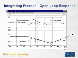
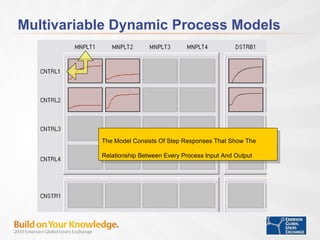
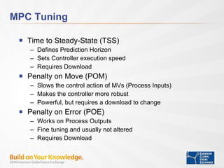
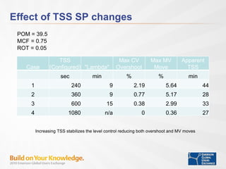
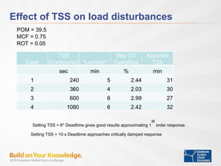
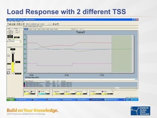
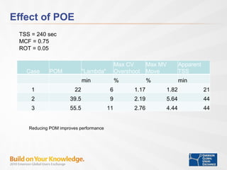
The document discusses controlling integrating processes like liquid levels using model predictive control (MPC). It explains that integrating processes require control since they have no natural equilibrium. The key points covered are: - MPC can effectively control integrating processes by considering feedback, model correction, rotation factors, and tuning parameters. - Tuning time to steady state, penalty on move, and model correction factor impact control performance for setpoint changes and load disturbances. - With proper tuning, MPC provides improved control of integrating processes compared to conventional PI control.


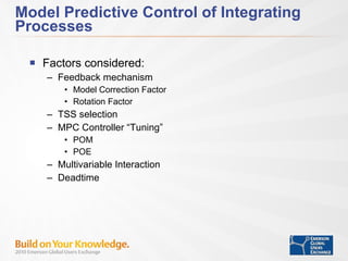
![Digital Signal Processing[ECEG-3171]-Ch1_L02](https://cdn.slidesharecdn.com/ss_thumbnails/dspl2-180427094423-thumbnail.jpg?width=640&height=640&fit=bounds)