.

1. 1B Erik Ydstie, CMU
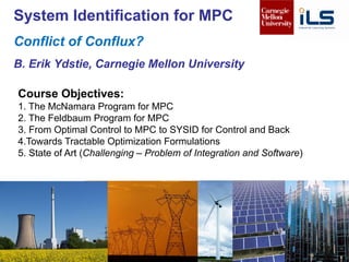
Course Objectives:
1. The McNamara Program for MPC
2. The Feldbaum Program for MPC
3. From Optimal Control to MPC to SYSID for Control and Back
4.Towards Tractable Optimization Formulations
5. State of Art (Challenging – Problem of Integration and Software)
System Identification for MPC
Conflict of Conflux?
B. Erik Ydstie, Carnegie Mellon University

2. System Identification (SYSID) Review
Mass and Energy Balance Constraints (nonlinear)
dzi
dt
=pi(z) +
nMV +nDVX
j=1
fi(uj, z), i = 1, ..., n
yk =hk(z), k = 1, ..., nP V
Linear (output) error model
e(t) = y(t) Gp(q 1
)u(t)
LT
Feed
Product
Cooling water return
FT
TT
Interface Layer (SCADA)
Measured
Outputs y
Control Inputs u
CT
FT
FT
Distributed Control System (DCS)
Setpoints y*
Model Predictive Controller
• Capture Flowsheet structure
• Energy and material balances
- Collinearity
- Uncollinearity
Used for very large systems
50 + MV/DVs 100+ CVs

3. B. Erik Ydstie, ILS Inc. 3
Data Flow
MPC
Control
ABB
Honeywell
Aspen
Emerson
Process
Prior Information
Step-response
State Space
Laguerre,…
Tuning Parameters,…
.XML
.TXT

4. B. Erik Ydstie
Model estimated using output error identification (global optimality)
MPC –SYSID
• Boiler Master –Turbine Master Controls (Emerson/Ovation)
• Turbine Controls for Siemens
SYSID Data from

5. B. Erik Ydstie

6. Problem: Define the Operator G that “best”
matches the prior information and process data.
Bayes Estimation Problem with Constraints
• Prior structure of G
• Digraph (edges in the process network)
• Parametric representation for each Gij (nodes)’
• Information of collinearity structure
• Process Data
• Semi-closed loop
• Experiment Design
G25
G38
0 1000 2000 3000 4000 5000 6000 7000
-50
0
50
100
150
200
250
300
350
400
Prior Information: System Strucure
10 MV/DVs
12 CVs
I/O Data
Digraph
Network
Collinearity:
SVD
RGA
Angles
N(n, m) =
(n 1)n(m 1)m
4
= 2970, 7! 0.12 deg separation
Bilinear constraints

7. Prior Information: Model Structures
B. Erik Ydstie, ILS Inc.
7
Polynomials used Name
B FIR, SR
A,B ARX, Equation error,
Instrumental variables,..
A,B,C ARMAX, AML
B,F OE (Output Error,
Markov-Laguerre, Kautz,…..)
State space representations have become popular for multivariable
systems after the introduction of sub-space identification.
Halfway Conclusion:
• The components are in place for systematic SYSID
• Software is lacking
• Quite difficult to do due to non-stationary disturbances
• Theory not that easy to understand completely
• Comprehensive Software solutions not available yet.

8. 8
n
CA
CA
CA
C
n
=
ú
ú
ú
ú
ú
ú
û
ù
ê
ê
ê
ê
ê
ê
ë
é
×
-1
2
rank
[ ] nBABAABB n
=× -12
||||rank
)(
)(
)(
)( tu
qA
qB
ty =
• A(q) and B(q) no common factors = Observable+Controllable (Co-prime)
• A(q) and B(q) no common unstable factors = Detectable+Stabilizable
Reachability: Any state can be
reached in a finite amount of time
Observability: Any
state can be
determined in a finite
amount of time
Detectable: Any unstable state is observable
Stabilizable: Any unstable state is reachable
The Admissibility Problem
The FIR / Markov-Laguerre Models are automatically stabilizable

9. B. Erik Ydstie, ILS Inc. 9
MISO Identification
Data is persistently excited from a SISO case.
0 500 1000 1500 2000 2500
-4
-2
0
2
4
6
8
10
12
14
16
MV7 is most excited
MV2 is least excited
Cond(F) = O(1)
1
N
NX
k=1
u(k)u(k i)
0 1000 2000 3000 4000 5000 6000 7000 8000 9000
-3
-2
-1
0
1
2
3
4
5
6
CV 3
Prior (blue)
Update (red)
Data (yellow)
Excitation
MV 1 D
MV2 A
MV3 A
MV 4 A
MV 5 A
MV 6 A
We get (Ljung, Wahlberg, Forsell) Bias and Variance:
Bias
Variance

10. B. Erik Ydstie, ILS Inc. 10
System
u1
u2
y1
y2
Generating Multivariable Input Signals
Same results hold as long as PE and independent noise and disturbance sequences.
Results based law of large numbers, difficult to achieve using PRBS type excitation.
1
N
NX
k=1
u(k)u(k i) = V (N)T
V (N i) = R(N) =
⇢
R > 0, i = 0
0, i 6= 0
Input sequences must be independent in time wrt to the network.
1 2 3 4 5 6 7 8 9 10
0
2
4
6
8
10
0 1000 2000 3000 4000 5000 6000 7000
28
30
32
34
36
38
40
42
44

0.2210 0.2206
0.2206 0.3301
[0.2019]
10
8
6
4
2
00
2
4
6
8
1
-0.5
0
0.5
10
Orthogonal inputs:
Mass balance
constraints in the
process

11. B. Erik Ydstie, ILS Inc. 11
y(t) = Gc
0(q 1
)u(t) + Hc
0(q 1
)v(t)
Gc
0(q 1
) = Sc
0(q 1
)G0(q 1
)
Hc
0(q 1
) = Sc
0(q 1
)H0(q 1
)
Sc
0(q 1
) =
1
1 + G0(q 1)K(q 1)
Closed Loop
System:
Issues for closed loop identification:
• Model parameterization
• Algorithm and mathematical approach
• Filters to shape bias and variance
• Excitation (complete theory for SISO, Lacking for MIMO, some progress for Networks
• Extension to multivariable case (treated very superficially in most books and papers)
Methods that may fail:
• Regression type models (equation error, instrumental variables)
• Subspace methods
• Compensation methods (direct and indirect)
• Correlation/spectral methods
Closed Loop Identification
Use output error methods for identification (open and closed loop)
Excitation
Process
MPC

12. 12
Integration of SYSID with MPC:
The Decision Problem
1. Defining clear business objectives (Stable/Robust Performance)
2. Developing plans to achieve the objectives (Predictive Control)
3. Systematically monitoring progress against the plan (Feedback, Filter)
4. Adapt objectives/plans as new needs and opportunities arise (Identification)
Control/Plan Process Measure
Robert McNamara,1960,
(CEO Ford, US Secretary of State)
Repeated Identification -> Iterative Learning -> Adaptive Control
Model and Desired Performance Objectives

13. 13
The McNamara Program for MPC
MPC Process Measure
Evaluate
Critic
Model and Desired Performance Objectives MPC Design/Identify/Adapt
1. Measure, evaluate and critique (Gap analysis)
2. Control strategies (Optimal Control/Model Predictive Control/Hinfinity)
3. Identification, Learning, Adaptation
a) Adapt Controllers (directly or indirectly)
b) Adapt Performance Objectives (closed loop, Q,R/move suppression)
Performance Objectives
Predictive Model
• The Decision problem is driven by Uncertainty (more than accurate models)
• Numerous Practical and Theoretical Challenges Remain
• MPC provides a fruitful Paradigm to Study these Challenges
Current Practice

14. B Erik Ydstie, CMU 14
The Feldbaum (1961) Program
Each field well advanced, but poorly integrated
(Especially on the software side)
min
u2U,y2Y
1X
i=1
(y(t + i + 1) y(t + i + 1)⇤
)2
+ ru(t + i)2
• Optimal (Certainty Equivalent, LQ Optimal Control, 1980 to MPC)
• Caution (Robust Control, 1980 )
• Probing (System ID / Adaptation, 1980 )
H1
min
u(t+i)
TX
i=0
ˆx(t + i)T
Qˆx(t + i) + u(t + i)T
Ru(t + i)
| {z }
Finite Horizon Cost
+ ˆx(t + i)T
P ˆx(t + i)
| {z }
Terminal Cost
Subject to: ˆx(t + 1) = Aˆx(t) + Bu(t)
ˆx(t + i)min  ˆx(t + i)  ˆx(t + i)max
u(t + i)min  u(t + i)  u(t + i)max
*
*

15. B Erik Ydstie, CMU 15
From LQ to MPC and Back Again
Step 2: Split Objective in Two and use Predictions from Model
Step 1: Formulate a (linear) model
Step 3: Ignore last part
Step 4: Solve QP and use first control.
Step 3: Repeat Step 4 (and hope for the best)
Theory for robust stability and performance
x(t + 1) = Ax(t) + Buf (t) + Ke(t)
ˆy(t) = ✓T
x(t) + Duf (t) + e(t)
x(t + T)T
PT x(t + T)
min
u2U,ˆy2Y
T 1X
i=0
(ˆy(t + i + 1) y(t + i + 1)⇤
)2
+ ru(t + i)2
| {z }
Model Predictive Control
+
1X
i=T
(ˆy(t + i + 1) y(t + i + 1)⇤
)2
+ ru(t + i)2
| {z }
LQ Control

16. B Erik Ydstie, CMU 16
MPC and SYSID:
Learn from the Past and Control Into the Future
Step 2B: Split Objective in Three and use Past Information
Model Identified from Past Data
Control Into the Future
min
✓2⇥
NX
i=0
(ˆy(t i) y(t i)⇤
)2
+ (✓ ✓0)T
F0(✓ ✓0)
| {z }
SYSID Bayes
min
u2U,ˆy2Y
1X
i=1
(ˆy(t + i + 1) y(t + i + 1)⇤
)2
+ ru(t + i)2
| {z }
Robust MPC
• Adaptive Control
• Iterative Control
• Closed Loop Identification
• Identification for Control
+++
Basic Idea: Controller works
while data is collected
✓(0) 7! ✓(t1) 7! ✓(t2), ....

17. SYSID and MPC - Conflict or Conflux?
Adapted from Polderman (1986)
Exampe: LTI System:
Linear feedback:
System
y(t) = ay(t 1) + bu(t 1)
e(t) = y(t) ˆy(t)
Model
+
-
Question: Will system satisfy performance specifications when the same
control is applied to both systems?
(The question of (Roust Lagrange) stability for closed loop identification and control was addressed by 1995)
u
y
u(t) = K(ˆa,ˆb)y(t)
Definition: An Identification Based Control is said to be Self-Tuning if SYSID
gives the “correct control”
Set of Identified Models : G
Set of Parameters with correct controls : H
Control and Estimation are Self Tuningif : H ✓ G

18. B Erik Ydstie, CMU 18
G = {ˆa,ˆb : ay(t 1) bK(✓)x(t)
| {z }
y(t)
= ˆay(t 1) ˆbK(✓)x(t)
| {z }
ˆy(t)
}
Analysis: Assume model output matches plant output
An infinite number of solutions. These depend on K.
Example 1: One step ahead predictive control
Solve for u(t) : y(t + 1)⇤
= ay(t) + bu(t)
G =
⇢
ˆa,ˆb :
a
b
=
ˆa
ˆb
u(t) =
ˆa
ˆb
y(t)
Get correct control even if
parameter estimates are off.
Thm: Any identifier that minimizes
prediction error is self tuning when used
with minimum variance control.
Admissibility Problem (close to singularity gives large, oscillatory controls)
(Problem of “direction”)
a
-1 -0.5 0 0.5 1
b
-1
-0.5
0
0.5
1
The admissible set

19. B Erik Ydstie, CMU 19
Example 2: Pole placement control (Vogel and Edgar,
Find gains so that : y(t) = a0y(t 1), 0 < a0 < 1
u(t) =
ˆa a0
ˆb
y(t)
H =
⇢
ˆa,ˆb :
a
b
y(t)) =
ˆa
ˆb
y(t)The set that gives
correct controls
H ✓ G
H =
⇢
ˆa,ˆb :
a a0
b
y(t)) =
ˆa a0
ˆb
y(t)
H ✓ G
Thm: Any identifier that minimizes
prediction error is self tuning when used
with pole-placement.
In this case Admissibility is more Complex as we
require:
Observability and Controllability
Can be expressed as Bilinear Constraints in
SYSID problem.
It is going well so far!!
a
-1 -0.5 0 0.5 1
b
-3
-2
-1
0
1
2
3
4
Admissible set

20. B Erik Ydstie, CMU 20
Example 3: Model Predictive Control
H =
⇢
ˆa,ˆb :
a a0
b
y(t)) =
ˆa a0
ˆb
y(t)
Thm: MPC does NOT satisfy the self-tuning principle.
min
u
(ˆy(t + 1)2
+ ru(t)2
) + py(t + 1)2
u(t) =
ba
r + b2
G =
(
ˆa,ˆb : a ˆa = (b ˆb)
ˆba
r + ˆb2
)
H 6✓ G
unless :
r = 0 and/or
ˆa = a, ˆb = b
-1 -0.5 0 0.5 1
-5
0
5
H
H
G

21. B Erik Ydstie, CMU 21
Problem: Information in the Past is Not Connected to Future Information
Additional means are needed to get optimal controls for MPC.
• Persistent Excitation to Converge Controls
• More Complex Controls to Align sets G and H?
• “Intelligent” Excitation (SYSID for Control, Dual Control)

22. B Erik Ydstie, CMU 22
From Feldbaum to MPC and Back
min
u2U,y2Y
TX
i=1
(y(t + i) y(t + i)⇤
)2
+ ru(t + i)2
| {z }
Model Predictive Control
+
1X
i=T +1
(y(t + i) y(t + i)⇤
)2
+ ru(t + i)2
| {z }
LQ Control
ˆy(t + i) Maximum Likelihood Estimate
F(t + i) Fisher Information Matrix
min
u2U,ˆy2Y
TX
i=1
(ˆy(t + i) y(t + i)⇤
)2
+ ru(t + i)2
| {z }
Robust CE AMPC
+ x(t + i)T
F(t + i) 1
x(t + i)
| {z }
Information Gathering
+x(t)PT x(t)
Challenges (identification using past data is the easiest):
• Solve a robust control problem on line (structured and unstructured uncertainty)
• “Back out control signals” from forward propagation of Fisher matrix
• What to do with the arrival cost

23. Special Case (TA Heirung/ J Morinelly)
• Fix the transition matrix A (step-response/Kautz model)
• Solve CE (rather than robust Hinfinity) control problem (caution
related to parameter uncertainty only)
• Ignore arrival cost
Computationally Expensive and Untested

24. 24
So What are the Issues?
Data Rich – But Information Poor Systems
(Nature is not a kind adversary)
• MPC and SYSID - Conflict or Conflux?
• How to represent/parametrize the system
• How to excite the system
• How to manage changing models
• Directionality
• Complexity
• Software

25. 25
Conclusions
• MPC is not self tuning
• There is a “strong" inter-action between
control and identification
• Different ways to “solve the problem”
– More complex “control”
– External Excitation (setpoints/inputs)
– Identification for control
• Need to Retune Controller when model
changes
• Collinearity issue is not well understood
• Very Large scale Applications are challenging
• MPC Maintenance is still challenging

26. 4756 lines
of assembly
code (1983)
15 lines
of MATLAB
code (2014)
CMU
Pitt
Golden Opportunities