This document discusses the use of model predictive control (MPC) to control the composition of a liquid column in a chemical plant. It provides background on MPC and how it can be used for multivariable processes like liquid columns. The document describes modeling a liquid column process in MATLAB Simulink and comparing the performance of MPC and PID control of the column. The results show that MPC provides better control of the column composition and liquid level than PID control.

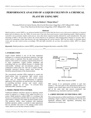
1. IJRET: International Journal of Research in Engineering and Technology eISSN: 2319-1163 | pISSN: 2321-7308
__________________________________________________________________________________________
Volume: 03 Issue: 05 | May-2014, Available @ http://www.ijret.org 127
PERFORMANCE ANALYSIS OF A LIQUID COLUMN IN A CHEMICAL
PLANT BY USING MPC
Babeeta Rathore1
, Manju Khare2
1
Pursuing M-Tech in Control System, Electrical & Electronics Engg Dept, LNCT, Bhopal M.P., India
2
Assoc Prof, Electrical & Electronics Engg Dept, LNCT, Bhopal M.P., India
Abstract
Model predictive control (MPC) is an advanced method of process control that has been in use in the process industries in chemical
plants and oil refineries since the 1980s. In recent years it has also been used in power system balancing models. Model predictive
controllers rely on dynamic models of the process, most often linear empirical models obtained by system identification. The main
advantage of MPC is the fact that it allows the current timeslot to be optimized, while keeping future timeslots in account. This is
achieved by optimizing a finite time-horizon, but only implementing the current timeslot. MPC has the ability to anticipate future
events and can take control actions accordingly. PID and LQR controllers do not have this predictive ability. MPC is a digital
control.
Keywords: Model predictive control (MPC); proportional-integral-derivative controller (PID)
---------------------------------------------------------------------***-----------------------------------------------------------------------
1. INTRODUCTION
Liquid column Method is one of the best separations
techniques in a chemical and petroleum industries, and tight
control action is important from the plant economics. The
purpose of the system is to separate a liquid mixture from two
or more components. Liquid Column modelling and
controlling both are very difficult because it’s dealing with
multivariable, nonlinear and non-stationary process. The
composition control plays the vital role in liquid columns.
Generally innovative process control tools increase the
flexibility and performance of the chemical plants.
The conventional controller (PID) employed to control the
liquid column does not guarantee tight control action
because it’s highly nonlinear. To solve critical control
issues and to achieve better performance in industrial
application, PID controllers are used but they face difficulties
in controlling non-linear process and cannot predict
immediate change in an input. To overcome these
difficulties MPC controller is used.
2. MODEL PREDICTIVE CONTROL
Traditional feedback controllers operate by adjusting control
action in response to a change in the output set point of a
system. Model predictive control (MPC) is a technique that
focuses on constructing controllers that can adjust the control
action before a change in the output set point actually occurs.
This predictive ability, when combined with traditional
feedback operation, enables a controller to make adjustments
that are smoother and closer to the optimal control action
values. Below we see the basic structure of MPC:
Fig 1: Basic structure of MPC
MPC consists of an optimization problem at each time
instants, k. The main point of this optimization problem is to
compute a new control input vector to be feed to the system,
and at the same time take process constraints into
consideration (e.g. constraints on process variables).
3. A BRIEF HISTORY OF INDUSTRIAL MPC
This section presents an abbreviated history of industrial MPC
technology. Figure 2 shows an evolutionary tree for the most
significant industrial MPC algorithms, illustrating their
connections in a concise way.

2. IJRET: International Journal of Research in Engineering and Technology eISSN: 2319-1163 | pISSN: 2321-7308
__________________________________________________________________________________________
Volume: 03 Issue: 05 | May-2014, Available @ http://www.ijret.org 128
Fig 2: Approximate genealogy of linear MPC algorithms
Model predictive control (MPC) technique started to be
implemented in industrial applications practically since
1970’s. The studies related with MPC initialized with Richalet
et al. (1978) as Model Predictive Heuristic Control (MPHC)
technique and named as Model Algorithmic Control (MAC).
The main characteristics of this type of controller include:
(1) The MPC controller attempts to optimize the process.
Dynamic models representing how the Process behaves are
used to predict future behavior and to determine the optimal
operating point.
(2) The predictions of the future behaviour are also used to
determine the control action taken by the controller.
Disturbances can be rejected before they affect the process.
(3) MPC is a multi-input, multi-output (MIMO) controller.
No input/output pairings need to be identified. All
manipulated variables are moved simultaneously to control all
the controlled variables. Interaction is accounted for with the
dynamic models and used as an advantage in the control. Also,
the number of inputs does not need to be equal to the number
of outputs. MPC can handle non-square systems very easily.
4. CONTROL OBJECTIVE FUNCTION OF MPC
There are several objective functions but, we applied
standard least-squares or quadratic programming objective
function. QP formulation gives smoother control actions and
the MPC will have more intuitive tuning parameters. The QP
formulation is used in this thesis. The objective function is a
sum of squares of the predicted errors (difference between the
set points and the model-predicted outputs) and the control
moves (changes in the control action from step to step).
A quadratic objective function for a predictive horizon of 3
and a control horizon of 2 can be written as.
      2
1
22
33
2
22
2
11   kkkkkkkk uRuRyˆrQyˆrQyˆrQ
Where yˆ represents the model predicted outputs, r is the
set point, ∆u is the change in manipulated input from one
sample time to the next, Q and R is a weight for the change
in the output and manipulated input respectively.
For a prediction horizon of P and a control horizon M,
the least square objective function is written as.
  



 
P
i
M
i
ikikik uRyˆrQ
1
1
0
22
The optimization problem solved is usually stated as a
minimization of the objective function, obtained by adjusting
the M control moves.
One limitation of output weight is we cannot take null matrix.
It can use step and impulse response data which can easily be
obtained.
4.1 MPC for MIMO Plants
One advantage of an MPC Toolbox design (relative to
classical multi-loop control) is that it generalizes directly to
plants having multiple inputs and outputs. Moreover, the plant
can be non-square, i.e., having an unequal number of actuators
and outputs. Industrial applications involving hundreds of
actuators and controller outputs have been reported.
5. SYSTEM DESCRIPTION
Figure 3 shows that the structure of a liquid column. The real
time data are taken from by using a reflux rate of the column
as kept constant and to give the sudden step changes of the
Reboiler temperature. The black box models can be
developed by correlating sequence relationship between
input and output data, here the input is Reboiler temperature
(manipulated variable) and the output is overhead product
composition (controlled variable). After obtaining the data
model has been developed by using a least square algorithm
(LS). The main application of least squares is model fitting.
Least square technique is mainly used for estimating the
system parameter and minimization of error so that here the
system parameter estimation and error minimization
developed by least square method it is one of the system
identification technique.

3. IJRET: International Journal of Research in Engineering and Technology eISSN: 2319-1163 | pISSN: 2321-7308
__________________________________________________________________________________________
Volume: 03 Issue: 05 | May-2014, Available @ http://www.ijret.org 129
Fig 3: Structure of Liquid Column
5.1 Modelling of Plant
The models used for the prediction in adaptive control to be
empirical input-output (Black-box) models. The main reason
for this is that input/output measurement data are available for
on-line estimation. These models fall under two major
categories: deterministic and stochastic. Deterministic
Models give a complete description of the plant response. In
practice these models tends to highly unrealistic since there
typically exist aspect that are out of our control. Stochastic
models contain some kind of random component usually
defined on a probability space. In this thesis we deal with
deterministic model. Let a system as a linear combination of
past output, y(k), and past input, u(k)
)mk(ub......)k(ub)k(ub)nk(ya.....)k(ya)k(y nn  11 101
Linear black box models can be obtained by ARX(Auto
Regressive exogenous), ARMAX(Auto Regressive Moving
Average exogenous) input etc.
5.2 SIMULINK Model in MATLAB:
Let we choose two variable w1 & w2 which is manipulated
outcomes of the two different controller PID and MPC. We
assume liquid column is filling with a chemical whose level
and concentration are too controlled by the controllers. Now
for this we have to design a plant which has two input w1 and
w2 also has two output level (h) and concentration (Cb). The
relation between input and output is
   
  












 2
1Cb
Cb
h
Cb2Cb2w
h
Cb1Cb1w
Cb 1.1
Cb1 and Cb2 are the maximum and minimum concentration
required for proper operation in liquid column. We choose
Cb1=24.9M and Cb2=0.1M.
 


1
h2.02w1wh 1.2
Height of the liquid in column is calculated by the equation
1.2. By using these two equations we design the process
model of the plant in MATLAB. Figure 4 shows the
SIMULINK model of Process Plant named as chemical plant
Fig 4: SIMULINK Model of using control of chemical plant
by PID or MPC
6. RESULTS AND DISCUSSION
A comparative analysis of the performance of the chemical
plant by both MPC and PID controller is obtained by
undergoing simulations in Matlab. The results show that MPC
is better controller than PID.
MPC controllers are probably the best assumption that can be
used for stable plants in the total absence of disturbance and
measurement information.
At 0s delay: figure 5 to 8 shows the variation in concentration
and level by PID or MPC.

4. IJRET: International Journal of Research in Engineering and Technology eISSN: 2319-1163 | pISSN: 2321-7308
__________________________________________________________________________________________
Volume: 03 Issue: 05 | May-2014, Available @ http://www.ijret.org 130
Fig 5: Concentration of liquid at 0s delays by PID controller
Fig 6: Concentration of liquid at 0s delays by MPC controller
Fig 7: Level of Liquid in Column at 0s delay by PID
Controller
Fig 8: Level of Liquid in Column at 0s delay by MPC
Controller
7. CONCLUSIONS
This Paper deals with the Model Predictive Controller and its
working in process control. It also shows that by an example
of liquid column it is the best methodology in advance process
control. Based on the comparison of the two control methods,
the process model MPC used to represent the system enables
MPC controller to predict the state of the plant during the
dynamic operation, which is particularly attractive as
compared with PID because the dynamics change as the water
level changes in the tanks, and a corresponding linearized
model of the water tank system can be used in real time by the
MPC.
REFERENCES
[1]. Allgower, F., & Zheng, A., (Eds.). (2000). Nonlinear
model predictive control, progress in systems and control
theory. Vol. 26. Basel, Boston, Berlin: Birkhauser Verlag.
[2]. Bartusiak, R. D., & Fontaine, R. W. (1997). Feedback
method for controlling non-linear processes. US Patent
5682309.
[3]. Kouvaritakis, B., & Cannon, M. (Eds.) (2001). Nonlinear
predictive control, theory and practice. London: The IEE.
[4]. Maciejowski, J. M. (2002). Predictive control with
constraints. Englewood Cliffs, NJ: Prentice Hall.
[5]. Martin, G., & Johnston, D. (1998). Continuous model-
based optimization. In Hydrocarbon processing’s process
optimization conference, Houston, TX.
[6]. Young, R. E., Bartusiak, R. B., & Fontaine, R. B. (2001).
Evolution of an industrial nonlinear model predictive
controller. In Preprints: Chemical process control—CPC VI,
Tucson, Arizona
[7]. Mayne, D. Q., Rawlings, J. B., Rao, C. V., & Scokaert, P.
O. M. (2000). Constrained model predictive control: Stability
and optimality.
[8]. MATLAB, Optimization and Control Toolbox,
www.mathworks.com