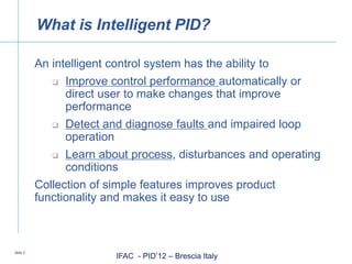
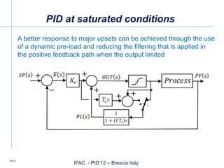
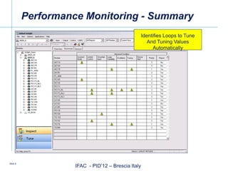
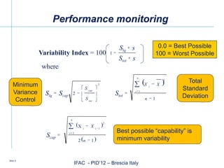
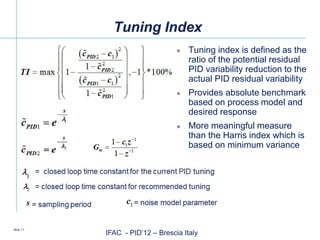
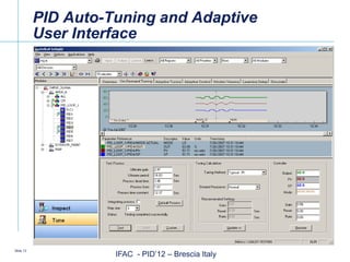
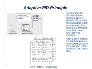
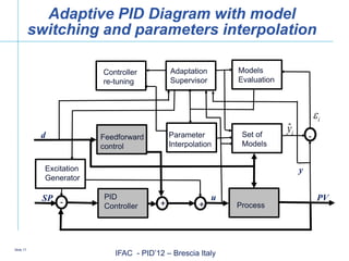
The document discusses advancements in intelligent PID (Proportional-Integral-Derivative) control systems presented at the IFAC conference in Brescia, Italy. It outlines features such as automatic performance improvement, fault detection, and an adaptive user interface that enhance control effectiveness. Key topics include PID tuning techniques, adaptive modeling, and the significance of robust process model identification for user acceptance.

1. Intelligent PID Product Design
IFAC Conference on Advances in PID Control
Brescia, 28-30 March 2012
Willy Wojsznis
Terry Blevins
John Caldwell
Peter Wojsznis
Mark Nixon
Slide 1 IFAC - PID’12 – Brescia Italy

2. What is Intelligent PID?
An intelligent control system has the ability to
 Improve control performance automatically or
direct user to make changes that improve
performance
 Detect and diagnose faults and impaired loop
operation
 Learn about process, disturbances and operating
conditions
Collection of simple features improves product
functionality and makes it easy to use
Slide 2
IFAC - PID’12 – Brescia Italy

3. PID controller options selection
Slide 3
IFAC - PID’12 – Brescia Italy

4. Nonlinear PID parameters
Slide 4
IFAC - PID’12 – Brescia Italy

5. PIDPlus for Wireless Communications
 To provide best control when a measurement is not updated on
periodic basis, the PID must be modified to reflect the reset
contribute for the expected process response since the last
measurement update.
 Standard feature of the PID in DeltaV for example
PIDPlus Design
Slide 5
IFAC - PID’12 – Brescia Italy

6. PID at saturated conditions
A better response to major upsets can be achieved through the use
of a dynamic pre-load and reducing the filtering that is applied in
the positive feedback path when the output limited
Slide 6
IFAC - PID’12 – Brescia Italy

7. Performance Monitoring- Overview
Slide 7
IFAC - PID’12 – Brescia Italy

8. Performance Monitoring - Summary
Identifies Loops to Tune
And Tuning Values
Automatically
Slide 8
IFAC - PID’12 – Brescia Italy

9. Performance monitoring
Slq + s 0.0 = Best Possible
Variability Index = 100 1- 100 = Worst Possible
Stot + s
where:
n
 (X ) Total
2
Minimum 2 - X
 S cap  i
Standard
Variance Slq = Scap 2 -   Stot = i =1
n -1 Deviation
Control  S tot 
n
 (X i - X
i -1
)2
i= 2 Best possible “capability” is
Scap = s - Sensitivity Factor
minimum variability
2 (n - 1 )
Slide 9
IFAC - PID’12 – Brescia Italy

10. Valve Diagnostics
• The approach uses the process model gain and is the best suited for
the adaptive control loops or automatically tuned loops where process
gain is known
• Valve stem position availability improves the diagnostics
• After calculating oscillation amplitudes on the controller input and
output, valve HYSTERESIS is defined directly as:
h = 2 A(out ) 2 Ampl ( PV ) = Kr
r = 2 Ampl ( PV ) b = h-r
K
Slide 10
IFAC - PID’12 – Brescia Italy

11. Tuning Index
 Tuning index is defined as the
ratio of the potential residual
PID variability reduction to the
actual PID residual variability
 Provides absolute benchmark
based on process model and
desired response
 More meaningful measure
than the Harris index which is
based on minimum variance
Slide 11
IFAC - PID’12 – Brescia Italy

12. PID Auto-Tuning and Adaptive
User Interface
Slide 12
IFAC - PID’12 – Brescia Italy

13. PID Graphical Gain-Phase Margin Tuning
Slide 13
IFAC - PID’12 – Brescia Italy

14. Adaptive PID Principle
 For a first order
Multiple Model
Interpolation with re-
Estimated
Gain, time
plus deadtime
centering constant, and process, twenty
deadtime seven (27) models
are evaluated each
Ke -TD sub-iteration, first
gain is determined,
1 + s then dead time,
Changing First Order Plus
process input Deadtime Process and last time
constant.
G1+ Δ G1+ Δ G1+ Δ  After each iteration,
TC1 -Δ TC1–Δ TC1 -Δ
G1 G1
DT1- Δ DT1
G1
DT1+ Δ the bank of models
TC1 -Δ TC1–Δ TC1 -Δ
G1-Δ DT1- Δ ΔDT1 Δ
G1- G1- DT1+ Δ is re-centered using
TC1 -Δ TC1–Δ TC1 -ΔΔ G1+ Δ
DT1- Δ DT1
G1+ Δ G1+
TC1 DT1+ Δ
TC1 TC1
the new gain, time
G1 DT1- Δ DT1 G1DT1+ Δ
TC1
G1
TC1 TC1
constant, and dead
G1-ΔDT1-G1- Δ G1- ΔDT1+ Δ
Δ DT1 time
TC1 TC1 Δ TC1 Δ G1+ Δ
G1+ G1+
DT1- Δ DT1 +Δ TC1+Δ TC1 +Δ
TC1 DT1+ Δ
G1 DT1- Δ DT1 G1 DT1+ Δ
G1
TC1 +Δ TC1+Δ TC1 +Δ
G1-ΔDT1-G1- Δ G1- ΔDT1+ Δ
Δ DT1
TC1 +Δ TC1+Δ TC1 +Δ
DT1- Δ DT1 DT1+ Δ
Slide 14
IFAC - PID’12 – Brescia Italy

15. Adaptive modeling with parameter
interpolation
•Every parameter value of the model is evaluated
independently
•The weight assigned to the parameter value is inverse of
the squared error
•Adapted parameter value is weighted average of all
evaluated values – decrease the number of models
dramatically
•Interpolation delivers improved accuracy, compared to
selection from the limited number of models
Slide 15
IFAC - PID’12 – Brescia Italy

16. Sequential Parameter Interpolation
•Sequential parameter adaptation – less models:
Model with 3 parameters (Gain, Lag, Dead Time) and 3 values for every
3
parameter has 3 model variations for model switching adaptation
or 3x3 model variations for sequential parameter adaptation
•Using the original data and Gain
performing adaptation iteratively Dead time
Initial
model
•
3
1
Final
The procedure on-line practically 2 model
feasible with sequential adaptation
Lag
Slide 16
IFAC - PID’12 – Brescia Italy

17. Adaptive PID Diagram with model
switching and parameters interpolation
Controller Adaptation Models
re-tuning Supervisor Evaluation
i
ˆ
yi
d Feedforward Parameter Set of -
control Interpolation Models
Excitation y
Generator
SP - PID u PV
Controller + + Process
Slide 17
IFAC - PID’12 – Brescia Italy

18. Adaptive modeling and control
Slide 18
IFAC - PID’12 – Brescia Italy

19. Adaptive model scheduling
Slide 19
IFAC - PID’12 – Brescia Italy

20. Conclusions
 The PID intelligence is commonly accepted by users with
various level of control expertise
 The main factor that contributed to the intelligent PID
acceptance is robust process model identification
 A significant factor is friendly user interface that provides
full insight into control loop operation, control
performance, loop faults and tuning recommendations
 Evolution of PID design will continue. PID will be facing
more challenges and deliver more successes.
Slide 20
IFAC - PID’12 – Brescia Italy

21. Acknowledgments
•Our communication with professors Karl Åstrӧm, Dale
Seborg and Thomas Edgar greatly improved the product
concepts and design.
•The final shape of the product and its quality is the result of
contributions from many control software developers –just to
name the core of the group:
Dennis Stevenson, John Gudaz, Peter Wojsznis, Mike Ott,
Yan Zhang and Ron Ottenbacher.
Slide 21
IFAC - PID’12 – Brescia Italy