This document provides an overview of model predictive control (MPC) and demonstrates its implementation in MATLAB using a continuous stirred tank heater (CSTH) model. It discusses key MPC concepts like observability, controllability, designing an observer, and formulating the optimization problem. MATLAB files and GUIs are also described that allow simulation and analysis of MPC behavior compared to traditional PID control.

1. Model Predictive Control for a Linearised Continuous
Stirred Tank Heater
or
MPC for Dummies
Sebastian Gonzato
September 2, 2016
Abstract
This report gives a brief overview of model predictive control and demonstrates how
it can be implemented in MATLAB. It is meant to be used as an accompaniment to the
MATLAB files and GUIs that were also produced for this project. A continuous stirred
tank heater model is used to illustrate key concepts such as observability, controllability,
designing an observer and formulating the optimisation problem. Insight into MPC
behaviour and a comparison with traditional PID control is also provided, The purpose
of this report is to introduce the inexperienced reader to MPC and hence the focus is
not on mathematical rigour.
1

2. Contents
1 Introduction 3
1.1 Scope of this report . . . . . . . . . . . . . . . . . . . . . . . . . . . . . . . . 3
1.2 Suggested prior knowledge . . . . . . . . . . . . . . . . . . . . . . . . . . . . . 3
1.3 MPC and its advantages . . . . . . . . . . . . . . . . . . . . . . . . . . . . . . 4
1.4 Overview of controlled system . . . . . . . . . . . . . . . . . . . . . . . . . . . 4
2 Observability & Controllability 6
2.1 Observability . . . . . . . . . . . . . . . . . . . . . . . . . . . . . . . . . . . . 6
2.2 Controllability . . . . . . . . . . . . . . . . . . . . . . . . . . . . . . . . . . . 7
3 Designing an Observer 8
3.1 Accurate state estimation . . . . . . . . . . . . . . . . . . . . . . . . . . . . . 8
3.2 Incorporating disturbance . . . . . . . . . . . . . . . . . . . . . . . . . . . . . 9
3.3 Incorporating time delay . . . . . . . . . . . . . . . . . . . . . . . . . . . . . . 10
4 Formulating optimisation 11
4.1 Regulation . . . . . . . . . . . . . . . . . . . . . . . . . . . . . . . . . . . . . . 11
4.2 Tracking . . . . . . . . . . . . . . . . . . . . . . . . . . . . . . . . . . . . . . . 13
4.3 Adding slew rate . . . . . . . . . . . . . . . . . . . . . . . . . . . . . . . . . . 15
4.4 Constraints . . . . . . . . . . . . . . . . . . . . . . . . . . . . . . . . . . . . . 16
5 Additional MATLAB resources 17
5.1 MATLAB scripts . . . . . . . . . . . . . . . . . . . . . . . . . . . . . . . . . . 17
5.2 GUIs . . . . . . . . . . . . . . . . . . . . . . . . . . . . . . . . . . . . . . . . . 17
5.2.1 Opening GUI . . . . . . . . . . . . . . . . . . . . . . . . . . . . . . . . 17
5.2.2 GUI features . . . . . . . . . . . . . . . . . . . . . . . . . . . . . . . . 18
5.2.3 Observer features . . . . . . . . . . . . . . . . . . . . . . . . . . . . . . 18
5.2.4 MPC features . . . . . . . . . . . . . . . . . . . . . . . . . . . . . . . . 18
6 Analysis of MPC controller 19
6.1 MPC behaviour . . . . . . . . . . . . . . . . . . . . . . . . . . . . . . . . . . . 19
6.1.1 Default behaviour . . . . . . . . . . . . . . . . . . . . . . . . . . . . . 19
6.1.2 Decreasing Q . . . . . . . . . . . . . . . . . . . . . . . . . . . . . . . . 20
6.1.3 Increase S . . . . . . . . . . . . . . . . . . . . . . . . . . . . . . . . . . 21
6.1.4 Decrease horizon . . . . . . . . . . . . . . . . . . . . . . . . . . . . . . 22
6.2 Comparison of MPC with PID controller . . . . . . . . . . . . . . . . . . . . . 23
7 Acknowledgements 25
2

3. 1 Introduction
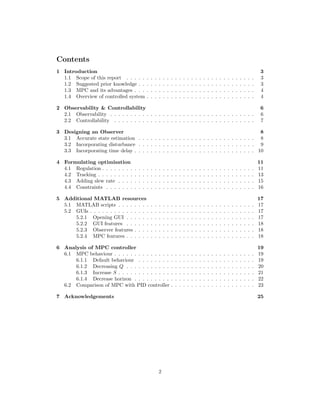
1.1 Scope of this report
The purpose of this report is to provide the reader with a basic grasp of model predic-
tive control (MPC). Specifically, this report covers why MPC is superior to traditional PID
controllers, some of the theory behind it and how to implement it in MATLAB using the
quadratic optimisation function quadprog. It is not supposed to be an in depth introduction
to MPC and hence few derivations are provided and mathematical rigour is sidelined.
Given that the author learned all of this reports contents in 6 weeks, there are undoubt-
edly mistakes in what follows. If the reader does use this report to implement a basic MPC
controller in MATLAB (or another capable language such as Python) they are advised to
read this report critically and not just take what is written for granted.
All the resources mentioned in this report (such as MATLAB files) can be found on the
Imperial College Centre for Process Systems Engineering web page [1].
1.2 Suggested prior knowledge
The theory behind MPC may be confusing to the reader with only a basic grasp of
control theory. Due to this, it is suggested that the reader spend some time learning about
the following topics:
• State space models and how they are derived [2]
• Behaviour of state space models [3]
• Conversion from continuous time to discrete time models [4]
The first two links come from online resources on modelling and control [2] provided by
Anthony Rossiter of the University of Sheffield. The author generally found these to be
useful and hence recommends them. The author also suggests watching the videos on ¢2
speed to save time and discourage lethargy.
The reader may also want to brush up on linear algebra and matrix properties. These
areas caused the author a lot pain, so a working knowledge of these will make the derivations
and equations that follow easier to understand and to derive independently. Many resources
are available online and the author recommends Khan Academy [5] and this NYU page [6]
for the properties of transpose matrices.
3

4. 1.3 MPC and its advantages
Traditional PID controllers are adequate for many simply systems and have been around
for more than a century (the first PID controller was implemented in 1911 [7]). Due to their
simplicity, they are still the most widely used controllers in industry. However, PID con-
trollers are fairly crude in that they are reactionary, and hence cannot be used to control
very complex systems such as say, cars. They also cannot handle constraints, which can be
very important if the output of a system (such as the temperature of an exothermic reaction
mixture) cannot go above a certain value.
To control complex systems while handling constraints requires knowledge of the con-
trolled system, hence the creation of model predictive control (MPC). The theory under-
pinning MPC first appeared in the 1960s and MPC itself has been in use in the chemical
processes industry since the 1980s. The basic idea behind MPC is that a model of the sys-
tem is used to make predictions and then the controller optimises the input to the system
to minimise error, control moves, slew rate or any other specification.
It should be noted that MPC is a way of thinking about or approaching control, and
hence there are many ways of implementing it. This means there are a range of control al-
gorithms that fall under the umbrella of MPC, such as predictive functional control (PFC),
generalised predictive control (GPC) which was developed by David Clarke of Cambridge
and David Mayne of Imperial, as well as many others. The key thing to bear in mind is
that in MPC the controller is not just reacting to the output of the system, but using that
output to make predictions and determine the best possible way of reaching a set point as
defined by the user.
1.4 Overview of controlled system
In process control it is important to have an understanding of the system being con-
trolled as this leads to good control decisions and makes troubleshooting easier.
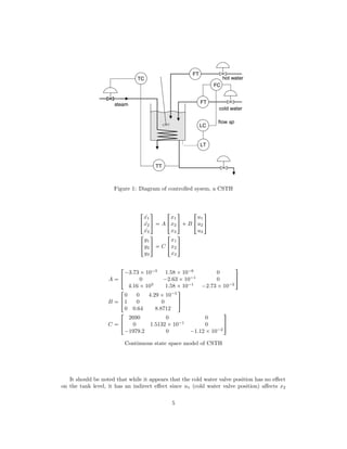
The system being controlled is a continuous stirred tank heater (CSTH, see Figure 1)
studied by Thornhill et al[8] which is composed of a tank, a steam heater, hot and cold
water valves and an outlet. The outlet valve is fully open and hence the flow is gravity
controlled.
This system exhibits many non linearities due to, for example, the heating coil occupying
volume and the density of water being a function of temperature. Since non linear MPC is
beyond the scope of this report, a linear model for the CSTH was used. The model, taken
from the same paper by Thornhill et al [8], was obtained by linearising around the operating
point shown in Table 1. The system is described by the state space model shown below,
where the variables are deviations from the operating point (i.e. x1 is actually ∆x1)
4

5. Figure 1: Diagram of controlled sysem, a CSTH
!
9x1
9x2
9x3
(
) A !
x1
x2
x3
(
) B !
u1
u2
u3
(
)
!
y1
y2
y3
(
) C !
x1
x2
x3
(
)
A !
¡3.73 ¢10¡3
1.58 ¢10¡6
0
0 ¡2.63 ¢10¡1
0
4.16 ¢103
1.58 ¢10¡1
¡2.73 ¢10¡2
(
)
B !
0 0 4.29 ¢10¡5
1 0 0
0 0.64 8.8712
(
)
C !
2690 0 0
0 1.5132 ¢10¡1
0
¡1979.2 0 ¡1.12 ¢10¡2
(
)
Continuous state space model of CSTH
It should be noted that while it appears that the cold water valve position has no effect
on the tank level, it has an indirect effect since u1 (cold water valve position) affects x2
5

6. Variable Description Range Operating point
x1 Volume of water, L 0 ¡8 3.3
x2 Cold water valve output, mA 4 ¡20 12.96
x3 Total enthalpy in tank, kJ 0 ¡3000 589
u1 Cold water valve position, mA 4 ¡20 12.96
u2 Steam valve position mA 4 ¡20 6.053
u3 Hot water valve position, mA 4 ¡20 5.5
y1 Level measurement, mA 4 ¡20 12
y2 Cold water flow rate measurement, mA 4 ¡20 7.33
y3 Temperature measurement, mA 4 ¡20 10.5
Table 1: Operating point
(cold water valve output) which in turn affects x1 (the tank level).
The model above describes the CSTH in continuous time. MPC however requires a
discrete time model since all computation takes a finite amount of time (a continuous MPC
controller would require the ability to perform computations in an infinitesimally short
time). The mathematics required to convert a continuous model to a discrete one are not
especially difficult, but fortunately MATLAB makes even this unnecessary and hence this
discretisation is covered in the MATLAB files but not in this report.
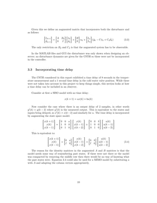
The system also exhibits a time delay of 1 second on the cold water valve position u1
and 8 seconds on the temperature measurement y3. While the MATLAB scripts and GUIs
were produced without taking this time delay into account, section 3.3 illustrates how to
incorporate this.
2 Observability Controllability
A summary of controllability and observability for state space models is presented be-
low. For more information the reader is directed to Anthony Rossiter’s videos on state space
model behaviour [3].
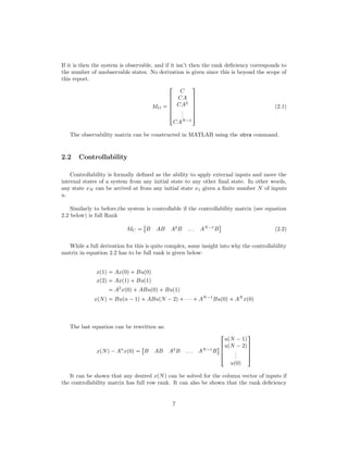
2.1 Observability
In order to predict the future outputs of a system, the states of that process (e.g. en-
thalpy, total mass) have to be known or observable. This is done by estimating them from
the outputs of the system, which in this case would be the level, temperature or cold water
flow rate. Loosely speaking then a system is said to be observable if it is possible to deter-
mine the behaviour of the system from it’s outputs.
With a state space model it is easy to determine whether a system is observable. Simply
construct the observability matrix from equation 2.1 and determine whether it is full rank.
6

7. If it is then the system is observable, and if it isn’t then the rank deficiency corresponds to
the number of unobservable states. No derivation is given since this is beyond the scope of
this report.
MO
!
C
CA
CA2
...
CAN¡1
(
0
0
0
0
0
)
(2.1)
The observability matrix can be constructed in MATLAB using the obvs command.
2.2 Controllability
Controllability is formally defined as the ability to apply external inputs and move the
internal states of a system from any initial state to any other final state. In other words,
any state xN can be arrived at from any initial state x1 given a finite number N of inputs
u.
Similarly to before,the system is controllable if the controllability matrix (see equation
2.2 below) is full Rank
MC
B AB A2
B . . . AN¡1
B
$
(2.2)
While a full derivation for this is quite complex, some insight into why the controllability
matrix in equation 2.2 has to be full rank is given below:
xp1q Axp0q Bup0q
xp2q Axp1q Bup1q
A2
xp0q ABup0q Bup1q
xpNq Bupn ¡1q ABupN ¡2q ¤¤¤ AN¡1
Bup0q AN
xp0q
The last equation can be rewritten as:
xpNq¡An
xp0q
B AB A2
B . . . AN¡1
B
$
!
upN ¡1q
upN ¡2q
...
up0q
(
0
0
0
)
It can be shown that any desired xpNq can be solved for the column vector of inputs if
the controllability matrix has full row rank. It can also be shown that the rank deficiency
7

8. of MC corresponds to the number of uncontrollable states.
As with observability, there is a MATLAB function to compute the controllability ma-
trix, namely ctrb.
3 Designing an Observer
This section looks at how to design an observer that allows the states of a system to
be determined. For more information on the subject the reader is referred to Anthony
Rossiter’s videos on state space observers [2].
3.1 Accurate state estimation
In order to control a process, the states of the controlled system must be known. This
is achieved using an observer which estimates the states using a model of the system. Cru-
cially, the observer includes an offset term which is defined as the difference between the
process output and the model output. Note that an observer can only ever estimate our
states since there will always be noise, measurement error and disturbances that we cannot
account for.
In the absence of a disturbance, the observer is defined as:
ˆxk 1 Aˆxk Bˆuk Lpyk ¡ ˆykq (3.1)
ˆyk Cˆxk
We can easily obtain ˆyk by multiplying our state ˆxk by the matric C, while our process
output yk can be measured directly. A hat on top of a variable indicates that it is a model
and not a process variable, although this distinction is dropped after this section.
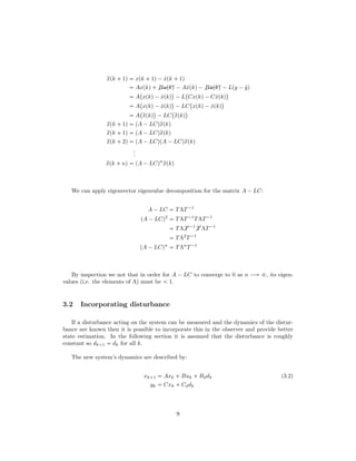
The matrix L has to be defined in order to guarantee offset free tracking. Specifically, it
has to be defined such that the eigenvalues of the matrix below are within the unit circle:
A ¡LC
The derivation for why this is can be found below. Note that qxpkq is simply a variable
we define as being the difference between our process states and our model states. If we
want offset free tracking qxpkq has to tend to 0 as n ÝÑ V.
8

9. qxpk 1q xpk 1q¡ ˆxpk 1q
Axpkq $$$Bupkq ¡Aˆxpkq¡$$$Bˆupkq ¡Lpy ¡ ˆyq
A
xpkq¡ ˆxpkq
¨
¡L
Cxpkq¡Cˆxpkq
¨
A
xpkq¡ ˆxpkq
¨
¡LC
xpkq¡ ˆxpkq
¨
A
qxpkq
¨
¡LC
qxpkq
¨
qxpk 1q pA ¡LCqqxpkq
qxpk 1q pA ¡LCqqxpkq
qxpk 2q pA ¡LCqpA ¡LCqqxpkq
...
qxpk nq pA ¡LCqn
qxpkq
We can apply eigenvector eigenvalue decomposition for the matrix A ¡LC:
A ¡LC TΛT¡1
pA ¡LCq2
TΛT¡1
TΛT¡1
TΛ T ¡1
T ΛT¡1
TΛ2
T¡1
pA ¡LCqn
TΛn
T¡1
By inspection we not that in order for A ¡ LC to converge to 0 as n ÝÑ V, its eigen-
values (i.e. the elements of Λ) must be 1.
3.2 Incorporating disturbance
If a disturbance acting on the system can be measured and the dynamics of the distur-
bance are known then it is possible to incorporate this in the observer and provide better
state estimation. In the following section it is assumed that the disturbance is roughly
constant so dk 1 dk for all k.
The new system’s dynamics are described by:
xk 1 Axk Buk Bddk (3.2)
yk Cxk Cddk
9

10. Given this we define an augmented matrix that incorporates both the disturbance and
as follows:
ˆxk 1
ˆdk 1
A Bd
0 I
ˆxk
ˆdk
B
0
uk
Lx
Ld
pˆyk ¡Cˆxk Cd
ˆdkq (3.3)
The only restriction on Bd and Cd is that the augmented system has to be observable.
In the MATLAB files and GUI the disturbance was only shown when designing an ob-
server; no disturbance dynamics are given for the CSTH so these were not be incorporated
in the controller.
3.3 Incorporating time delay
The CSTH considered in this report exhibited a time delay of 8 seconds in the temper-
ature measurement and a 1 second time delay in the cold water valve position. While these
were not taken into account in this project to keep things simple, this section looks at how
a time delay can be included in an observer.
Consider at first a SISO model with no time delay:
xpk 1q axpkq bupkq
Now consider the case where there is an output delay of 2 samples, in other words
yIpkq ypk ¡ 2q where yIpkq is the measured output. This is equivalent to the states and
inputs being delayed, so xIpkq xpk¡2q and similarly for u. The time delay is incorporated
by augmenting the state space model:
!
xpk 1q
xpkq
xpk ¡1q
(
) !
0 0 a
1 0 0
0 1 0
(
) !
xpkq
xpk ¡1q
xpk ¡2q
(
) !
0 0 b
1 0 0
0 1 0
(
) !
upkq
upk ¡1q
upk ¡2q
(
)
This is equivalent to:
!
xpk 1q
xpkq
xpk ¡1q
(
)
0 a
I 0
!
xpkq
xpk ¡1q
xpk ¡2q
(
)
0 b
I 0
!
upkq
upk ¡1q
upk ¡2q
(
) (3.4)
The reason for the identity matrices in the augmented A and B matrices is that the
model needs some way of remembering past states. If these were not there or the model
was compacted by removing the middle row then there would be no way of knowing what
the past states were. Equation 3.4 could also be used for a MIMO model by substituting a
with A and adapting the column vectors appropriately.
10

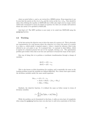
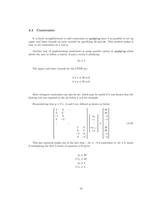
11. 4 Formulating optimisation
4.1 Regulation
In a tracking problem, the objective is to drive the states x of a system to 0. The
objective function J in this case then is:
J
N¸
i1
¢
xT
i Qxi uT
i Rui
(4.1)
where Q and R are weighting matrices.
The first term in equation 4.1 is fairly obvious; this term ensures that the controller
attempts to drive the error to 0. However, this term on its own leads to unreasonably large
actuator changes and can also lead to divergent input signals. This is because the best way
to punish the errors is simply to invert the plant (so the controller is just the inverse of the
plant model) which is not usually a good idea! [9]
Due to this, a second term in the equation 4.1 is need which punishes the number of
moves the controller makes which are away from it’s final steady state input.
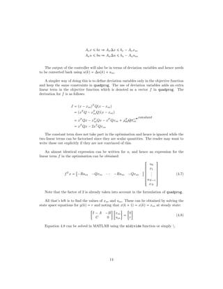
The MATLAB files and GUI produced for this project used the quadprog function to
solve equation 4.1. This function requires inputs of a paricular form as shown in equation
4.2 and hence we need to define matrices H, Aeq and beq.
minimize
x
1
2
xT
Hx fT
x
subject to Aeqx beq
Ax ¤ b
(4.2)
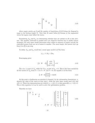
For tracking the vector f will just be a vector of zeros.
In order to proceed, the first thing to note is that in the optimisation, the x in quadprog
is not our state but actually the augmented vector:
!
u0
x1
...
uN¡1
xN
(
0
0
0
0
0
)
where N is the prediction horizon, xi
xi,1 xi,2 xi,3
$T
and similarly for u. The first
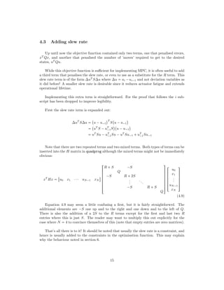
element u0 is required when defining constraints and is also useful later when an extra term
in the objective function is added in order to punish the slew rate pui ¡ui¡1q.
From this, the formulation of H is fairly simple:
11

12. H
!
R
Q
R
Q
...
(
0
0
0
0
0
)
(4.3)
where empty entries are 0 and the number of repetitions of Q, R along the diagonal is
equal to the horizon length N. Note that R comes before Q because in the augmented
vector the inputs come before the states.
Formulating Aeq and beq (or determining whether they are needed at all) is less obvi-
ous. The equality constraint is needed since our objective function has to satisfy system
dynamics; the state space model determines what routes or sequence of inputs can get the
controlled system from one set of states to another. Put more simply, the system can’t go
from A to B in one step.
To define Aeq and beq recall that a state space model is of the form:
xk 1 Axk Buk
Rearranging gives:
A B ¡I
$
!
xpkq
upkq
xpk 1q
(
) 0 (4.4)
The r.h.s. is part of Aeq while the l.h.s. is part of beq 0. This is the form needed for
all the entries of Aeq from k 1 to k N. For k 0, the equality is of the form:
¡B I
$
up0q
xp1q
Axp0q (4.5)
At this point a clarification on notation is required. In the optimisation formulation, xi
denotes the value of the states at time step i, while the state space model used xpkq and
xpk 1q. These two representations are related; x1 xpk 1q or more generally xi xpk iq.
This is why equation 4.4 can be used to solve the optimisation problem.
Therefore we have:
!
¡B I
A B ¡I
A
...
A B ¡I
(
0
0
0
0
0
0
0
0
0
)
!
u0
x1
u1
x2
...
xN¡1
uN¡1
xN
(
0
0
0
0
0
0
0
0
0
0
0
)
!
Ax0
0
...
...
...
0
(
0
0
0
0
0
0
0
0
0
)
(4.6)
12

13. where as noted before xi and ui are vectors for a MIMO system. From inspection it can
be seen that the matrix on the r.h.s is Aeq and the vector on the l.h.s. is beq. Care should be
taken when defining the equality in MATLAB since while only single zeros or empty entries
(which also correspond to zeros) are shown in equation 4.6, these are actually null matrices
whose size needs to be specified in MATLAB.
And that’s it! The MPC problem is now ready to be coded into MATLAB using the
quadprog function.
4.2 Tracking
In the last section the objective was to drive the states of a system to 0. This is obviously
not representative of a real process where the objective is to drive the states of a system
to a value xss which satisfy a required output r, where r stands for reference (this is also
referred to as a set point or sp). It is assumed that r is constant in what follows, which
is typical of a chemical process but not of, for example, driving a car. The optimisation
problem gets trickier when this is not the case and hence is beyond the scope of this report.
One way of doing this is to perform a coordinate transformation through a change of
variables:
∆xpkq xpkq¡xss
∆upkq upkq¡uss
This is also known as delta formulation for tracking, and is essentially the same as the
tracking problem except the variables are defined differently. For a linear state space model,
the deviation variables satisfy the same model equations:
∆xk 1 xpk 1q¡xss
Axpkq Bupkq¡pAxss Bussq
A∆xk B∆uk
Similarly, the objective function J is defined the same as before except in terms of
deviation variables:
J
N¸
i1
¢
∆xT
i Q∆xi ∆uT
i R∆ui
While the problem can be formulated in this form, it adds an extra layer of complexity
when using the quadprog function since you also have to add extra constraints of the form:
13

14. Axx ¤ bx ñ Ax∆x ¤ bx ¡Axxss
Auu ¤ bu ñ Au∆u ¤ bu ¡Auuss
The output of the controller will also be in terms of deviation variables and hence needs
to be converted back using upkq ∆upkq uss.
A simpler way of doing this is to define deviation variables only in the objective function
and keep the same constraints in quadprog. The use of deviation variables adds an extra
linear term in the objective function which is denoted as a vector f in quadprog. The
derivation for f is as follows:
J px ¡xssqT
Qpx ¡xssq
pxT
Q ¡xT
ssQqpx ¡xssq
xT
Qx ¡xT
ssQx ¡xT
Qxss $$$$$Xconstant
xT
ssQxss
xT
Qx ¡2xT
Qxss
The constant term does not take part in the optimisation and hence is ignored while the
two linear terms can be factorised since they are scalar quantities. The reader may want to
write these out explicitly if they are not convinced of this.
An almost identical expression can be written for u, and hence an expression for the
linear term f in the optimisation can be obtained:
fT
x
¡Russ ¡Qxss ¤¤¤ ¡Russ ¡Qxss
$
!
u0
x1
...
uN¡1
xN
(
0
0
0
0
0
)
(4.7)
Note that the factor of 2 is already taken into account in the formulation of quadprog.
All that’s left is to find the values of xss and uss. These can be obtained by solving the
state space equations for ypkq r and noting that xpk 1q xpkq xss at steady state:
I ¡A ¡B
C 0
xss
uss
0
r
(4.8)
Equation 4.8 can be solved in MATLAB using the mldivide function or simply .
14

15. 4.3 Adding slew rate
Up until now the objective function contained only two terms, one that penalised errors,
xT
Qx, and another that penalised the number of ’moves’ required to get to the desired
states, uT
Qu.
While this objective function is sufficient for implementing MPC, it is often useful to add
a third term that penalises the slew rate, or even to use as a substitute for the R term. This
slew rate term is of the form ∆uT
S∆u where ∆u ui ¡ui¡1 and not deviation variables as
it did before! A smaller slew rate is desirable since it reduces actuator fatigue and extends
operational lifetime.
Implementing this extra term is straightforward. For the proof that follows the i sub-
script has been dropped to improve legibility.
First the slew rate term is expanded out:
∆uT
S∆u
u ¡u¡1
¨T
S
u ¡u¡1
¨
uT
S ¡uT
¡1S
¨
u ¡u¡1
¨
uT
Su ¡uT
¡1Su ¡uT
Su¡1 uT
¡1Su¡1
Note that there are two repeated terms and two mixed terms. Both types of terms can be
inserted into the H matrix in quadprog although the mixed terms might not be immediately
obvious:
xT
Hx
u0 x1 ¤¤¤ uN¡1 xN
$
!
R S ¡S
Q
¡S R 2S
...
...
¡S R S
Q
(
0
0
0
0
0
0
0
)
!
u0
x1
...
uN¡1
xN
(
0
0
0
0
0
)
(4.9)
Equation 4.9 may seem a little confusing a first, but it is fairly straightforwrd. The
additional elements are ¡S one up and to the right and one down and to the left of Q.
There is also the addition of a 2S to the R terms except for the first and last two R
entries where this is just S. The reader may want to multiply this out explicitly for the
case where N 4 to convince themselves of this (note that empty entries are zero matrices).
That’s all there is to it! It should be noted that usually the slew rate is a constraint, and
hence is usually added to the constraints in the optimisation function. This may explain
why the behaviour noted in section 6.
15

16. 4.4 Constraints
It is fairly straightforward to add constraints in quadprog since it is possible to set up
upper and lower bounds on each variable by specifying lb and ub. This method makes it
easy to set constraints on u and y.
Another way of implementing constraints is using another option in quadprog which
allows the user to define a matrix A and a vector b satisfying:
Ax ¤ b
The upper and lower bounds for the CSTH are:
4 ¤ u ¤ 20 mA
4 ¤ y ¤ 20 mA
More stringent constraints can also be set, which may be useful if it was known that the
heating coil was exposed to the air below 8 mA for example.
Remembering that y Cx, A and b are defined as shown in below:
!
I 0 ¤¤¤
0 C
¡I 0
0 ¡C
...
...
I 0
0 C
¡I 0
0 ¡C
(
0
0
0
0
0
0
0
0
0
0
0
0
0
)
!
u0
x1
...
uN¡1
xN
(
0
0
0
0
0
)
¤
!
20
20
¡4
¡4
...
20
20
¡4
¡4
(
0
0
0
0
0
0
0
0
0
0
0
0
0
)
(4.10)
This last equation makes use of the fact that ¡Ax ¤ ¡b is equivalent to Ax ¥ b, hence
if multiplying the first 2 terms of equation 4.10 gives:
u0 ¤ 20
Cx1 ¤ 20
u0 ¥ 4
Cx1 ¥ 4
16

17. 5 Additional MATLAB resources
5.1 MATLAB scripts
As part of this report MATLAB scripts were produced to illustrate the various concepts
that were presented in this report, such as observability and solving the optimisation prob-
lem. These scripts are commented throughout to allow the user to better understand what
MATLAB is doing.
A description of what each script does is given below:
• MPC 1 Initial This script is run at the start of all subsequent scripts. It defines the
state space model of the CSTH and discretises it.
• MPC 2 Observer Defines an observer and plots its behaviour.
• MPC 3 Observerwithdisturbanceandnoise Similar to the previous script with the ex-
ception that a disturbance and noise is added to the process.
• MPC 4 Regulation MPC controller that drives states to 0 and plots the result.
• MPC 5 Tracking MPC controller that drives states to a defined reference state and
plots the result.
• MPC 6 Trackingwithslewandconstraints Similar to the previous script with the excep-
tion of an extra term in the objective function that penalises the slew rate as well as
the addition of constraints.
• PID Comparison Script used to compare PID behaviour in section 6.2
• Tf plant Simulink model of CSTH used in previous script.
5.2 GUIs
As part of this project two MATLAB GUIs were produced to illustrate the behaviour of
an observer and an MPC controller.
5.2.1 Opening GUI
The GUI is opened simply by double clicking the MATLAB .fig file. Make sure the func-
tion of the same name is in the same directory as the figure and do not rename anything!
If the GUI produces an error message when you open it, it may be necessary to first
open the GUI developer and construct the GUI before using it. To do this type guide in
the MATLAB workspace, choose the GUI you want to open then press the green arrow at
the top of the window or use Ctrl+T.
17

18. 5.2.2 GUI features
Some parameters are common to both GUIs, so these are considered below.
• Pole place This determines where the poles of A ¡ LC are placed in the unit circle.
The further this slider is to the right, the smaller the poles are and the faster the
observer response is, although the observer will also be more sensitive to noise.
• Noise This adds noise v to the measured output, where v appears in y Cx v. The
further to the right this slider is the higher the noise gain. The relationship between
the slider and the noise gain is non linear.
• Initial states This table determines the initial states of the actual plant and the ob-
server. These are set to the operating point by default.
• Timesteps This defines how many time steps the simulation runs for (remember MPC
has to be implemented in discrete time). The sample time for this MPC controller is
2 seconds.
• Run Runs simulation
5.2.3 Observer features
This GUI is called Observer 2 for historical reasons, and it was not changed since it is
annoyingly difficult to rename GUIs. Parameters other than the ones listed in section 5.2.2
are listed below.
• Disturbance The entries in this table determine the effect of a disturbance n the states
(Bd) and the output of the model (Cd). If you make one entry of Bd or Cd non-zero
they must all be non-zero!
5.2.4 MPC features
Parameters other than the ones listed in section 5.2.2 are listed below.
• Weightings These tables allow you to change the Q, R and S matrices
• Model mismatch This slider introduces a random model mismatch, so the model used
by the MPC controller is not the same as the actual process dynamics. The mismatch
is done by multiplying the model parameters by a randomly generated number and so
the mismatch is different each time the simulation is run.
• Set points This table allows you to change the set points at determined times. The
set point time changes are in timesteps (in this case 2 seconds) and not seconds. The
timesteps also need to be sequential i.e. you can’t have one set point change after
the next set point occurs. The GUI will still work but an error message should be
displayed in the workspace.
• Constraints This table allows you to define the constraints on the inputs as well as
the outputs.
• Horizon Use this box to set the prediction horizon and see how it affects the output.
18

19. 6 Analysis of MPC controller
Having designed an MPC controller in MATLAB, it is useful to analyse its behaviour in or-
der to obtain insights into how it behaves and why, as well as how it compares to traditional
PID control. In the sections that follow, this analysis was done for the step changes indi-
cated in table 2 and the controller horizon was 30 (unless otherwise stated). The observer’s
initial state was kept the same as that of the actual process.
Variable Description Initial Final
y1 Level measurement 12 mA 13 mA
y2 Cold water flow rate measurement 11.89 mA 10.5 mA
y3 Temperature measurement 10.5 mA 12 mA
Table 2: Set point changes for analysis of MPC behaviour
6.1 MPC behaviour
This section looks at how changing the weightings and event horizon affect controller
behaviour.
6.1.1 Default behaviour
The first simulation consisted of keeping the Q, R and S matrices as identity matrices.
The results are shown in figure 2.
Figure 2: Default behaviour
At these weightings, the level of the tank shoots up very quickly as the hot water valve
position is increased by 10 mA to compensate for the cold water valve closing and the
temperature set point being raised. Draining the tank takes a lot more time than filling
19

20. it up since the flow is gravity controlled, hence the slow decay to the set points after the
first move. The temperature takes as much time as the level to reach steady state since the
controller has made its moves such that once the tank is drained of the water that was there
initially, all the water will be at the right temperature.
The most noticeable aspect of figure 2 is that the controller only seems to do anything
in it’s first 2 moves, while the rest are pretty much constant save a few moves to ensure
0 steady state error. This can be seen quite clearly in figure 3 At these weightings, the
solution to the optimisation problem is to do everything at once in order to reduce the
penalty incurred by the xT
Qx term.
Figure 3: MPC inputs zoomed in
Evidently this is not desirable; having such rapid changes in controller outputs reduces
actuator life as well as the operational life of other components. These changes might also
have undesirable consequences that are not captured by the model; having the hot water
valve be opened so quickly might mean hot water splashing out of the tank for example.
6.1.2 Decreasing Q
To deal with this, the value of Q can be decreased. Figure 4 shows the results for when
Q is decreased by the amount shown in table 3.
Variable Description Weighting
u1 Cold water valve 10¡2
u2 Steam valve 10¡3
u3 Hot water valve 10¡3
Table 3: Q matrix weightings
The controller outputs are now much more reasonable; the hot water valve is making
a jump of only 3 mA in one move and similarly with the other 2 actuators. The system
20

21. Figure 4: MPC behaviour for reduced Q weighting
outputs are also smoother.
Decreasing Q entries further turns the MPC controller into a very basic predictive func-
tional control (PFC) controller in which the first value of u is chosen to be uss. PFC
controller’s of this form essentially maintain open loop dynamics, which is adequate if open
loop dynamics are desirable. This is not optimal however, and solving an optimisation prob-
lem only to end up with such a simple (and not particularly good) controller is as displeasing
as it is inefficient.
6.1.3 Increase S
There is still a significant slew rate for all 3 actuators which is undesirable. To overcome
this, the S weighting can be increased to the values shown in table 4. The results are shown
in 5.
Variable Description Weighting
u1 Cold water valve 102
u2 Steam valve 102
u3 Hot water valve 102
Table 4: S matrix weightings
This has not quite had the effect intended. While the slew rate for the hot water valve
has decreased it has only done so after it’s first move. Despite the relatively high weighting,
the same is true of all the other actuators which is problematic since the steam valve makes
a jump of roughly 3 mA in one move. No increase in the weighting of S can change this.
While the author cannot give an exact reason for why this is the case, it probably has
something to do with quadprog and how the optimisation problem is formulated. Adding
21

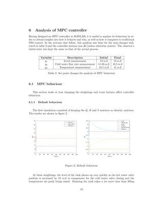
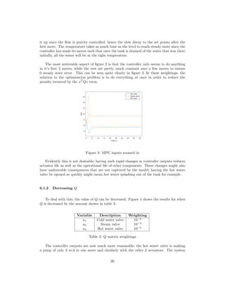
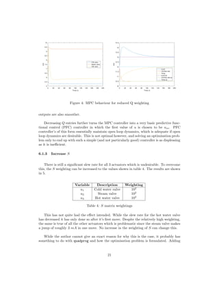
22. Figure 5: MPC behaviour for increased S weighting
the slew rate constraint in the constraints instead of the objective function could solve this.
Another solution to this would be to use the YALMIP toolbox to solve the optimisation
problem[10]. YALMIP is widely used in academia[11].
6.1.4 Decrease horizon
Figure 6 shows the MPC controller behaviour when the even horizon is decreased to 2
while keeping the same weightings as before.
Figure 6: MPC behaviour for a decreased event horizon
Disappointingly, this does not produce any notable changes in the MPC controller’s
behaviour other than a greater overshoot in the level. This can easily be explained by the
behaviour noted before, in that the slew rate of the MPC’s first move cannot be changed.
22

23. Manipulated variable Controlled variable
Hot water valve Level
Cold water valve Cold water flowrate
Steam valve Temperature
Table 5: PID setup
6.2 Comparison of MPC with PID controller
As the saying goes, ‘less is more’ and there’s no point using an MPC controller when
PID controllers are just as good.
In order to compare PID control with MPC, a SIMULINK file was created which con-
tained the linearised CSTH in transfer function form. PID controllers were added and used
to control the control variables as shown in table 5 They were then tuned independently to
provide reasonably good control.
Finally, the same step changes were used as shown in table 2. Normally decoupling
would be applied to minimise interactions, but in practice this did not matter as can be
seen in figure 7.
Figure 7: MPC behaviour (left) compared with 3 PID controllers in parallel (right)
If we’re only interested in settling time, the MPC controller appears to perform worse
than the 3 PID controllers! There is less overshoot in the level using PID controllers and a
significantly faster settling time for the level, although the settling time for the temperature
is roughly the same.
However, settling time is not the only important performance index. The inputs to the
system are also important, since these can change too rapidly (reducing actuator life) or
cause the actuator to saturate if the input is greater than 20 mA for example. Figure 8
23

24. compares the MPC inputs to the PID inputs.
Figure 8: Comparison of MPC and PID controller outputs
The steam valve jumps 12 mA in the first step which is undesirable due to the large slew
rate and because the valve is close to saturating.
Where MPC shines is in it’s ability to handle constraints, something PID controllers are
incapable of doing. Figure 9 shows a set point change only in the level from 12 mA to 20 mA.
Figure 9: Constraint handling behaviour of MPC illustrated by comparing MPC behaviour
(left) with PID behaviour (right)
The PID controller setup again has a slightly faster settling time for the level (roughly
60s compared to 100s for MPC), but it has a significant overshoot while the MPC does not.
If the PID controllers had been used to control the tank in real life, the tank would have
overflowed.
24

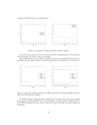
25. It should be noted that increasing the gain or decreasing the integral components of the
PI controller would lead to less overshoot and so less overflowing, but this would come at
the expense of a slower settling time.
7 Acknowledgements
I would like to thank Nina Thornhill of Imperial College London for agreeing to fund
this project despite it only being useful to me, and also for help throughout.
I would especially like to thank Harsh Shukla of EPFL for all the help he provided de-
spite being very busy with his PhD. Without him, this report would have been a very long
and boring text on how to implement GPC in Simulink.
References
[1] Gonzato, S. (2016). UROP MPC. [online] Nina Thornhill Imperial Col-
lege London Process Systems Personal Pages. Available at: http://personal-
pages.ps.ic.ac.uk/ nina/UROP/MPC.html [Accessed 1 Sep. 2016].
[2] Rossiter, A. (2016). Modelling and control. [online] Controleducation.group.shef.ac.uk.
Available at: http://controleducation.group.shef.ac.uk/indexwebbook.html [Accessed
29 Aug. 2016].
[3] Rossiter, A. (2016). state space behaviours - YouTube. [online] Youtube.com. Available
at: https://www.youtube.com/playlist?list=PLs7mcKy nInFCnBAMQanjRSLdLg6yWiuJ
[Accessed 29 Aug. 2016].
[4] Freeman, D. (2016). 2. Discrete-Time (DT) Systems. [online] YouTube. Available at:
https://www.youtube.com/watch?v=Ih4s5IFphCw [Accessed 29 Aug. 2016].
[5] Khan, S. (2016). Introduction to matrices. [online] YouTube. Available at:
https://www.youtube.com/watch?v=xyAuNHPsq-glist=PL26BD351D91DFB72E
[Accessed 29 Aug. 2016].
[6] Math.nyu.edu. (2016). The Basics: Properties of Matrices. [online] Available
at: http://www.math.nyu.edu/ neylon/linalgfall04/project1/dj/propofmatrix.htm
[Accessed 29 Aug. 2016].
[7] Building-automation-consultants.com. (2016). A Brief Building Automation His-
tory. [online] Available at: http://www.building-automation-consultants.com/building-
automation-history.html [Accessed 29 Aug. 2016].
[8] Thornhill, N., Patwardhan, S. and Shah, S. (2008). A continuous stirred tank heater
simulation model with applications. Journal of Process Control, 18(3-4), pp.347-360.
[9] Skogestad, S. and Postlethwaite, I. (1996). Multivariable feedback control. Chichester:
Wiley, pp.49-50.
25

26. [10] YALMIP : A Toolbox for Modeling and Optimization in MATLAB. J. Lfberg. In Pro-
ceedings of the CACSD Conference, Taipei, Taiwan, 2004.
[11] Harsh Shukla, 2nd
year PhD, EPFL, 2016.
26

27. Glossary
actuator fatigue Fatigue he weakening of a material caused by repeatedly applied loads
and is often the cause of actuator failure. 15
offset free tracking Offset free tracking means that the tracking (driving of states to 0)
of a controller does not produce an offset, i.e. there is no steady state error. The term
can also be used for observers tracking a systems states. 8
prediction horizon The event horizon of an MPC controller is the number of timesteps
into the future that the MPC controller considers when performing its optimisation.
11, 18
rank In linear algebra, the rank of a matrix A is the dimension of the vector space generated
(or spanned) by its columns. A matrix is full row rank if the rows are linearly indepen-
dent of each other, meaning you cannot produce one row from a linear combination
(through addition or multiplication) of the other rows. 6, 7
27