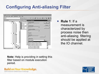
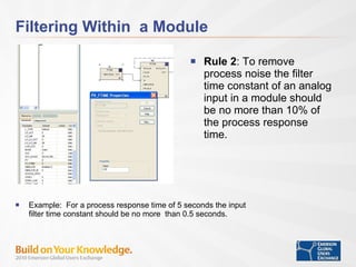
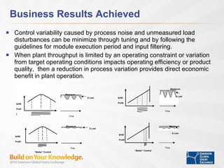
Guidelines for Setting Filtering and Module Execution Rate Terry Blevins  Principal Technologist
Presenters Terry Blevins, Principal Technologist  Kent Burr, Gary Law, Joe Nelson  – DeltaV Product Engineering
Introduction Filtering and module execution period can directly impact control performance.  In this workshop we will  be addressing: Protection against 50-60hz pickup provided by analog input card and Charm analog input. Filtering of process measurements –configuration guideline to void aliasing and to minimize impact of process noise. Control execution – configuration guideline for setting execution period based on process dynamics, impact on control performance. Guidelines for setting filtering and execution period are presented  and examples used to illustrate their impact.
Protection against 50-60 Hz pickup The DeltaV analog input card uses a two pole hardware (RC) filter to provide -3 dB at 2.7 Hz and  >  -40dB attenuation at 50-60 Hz. The CHARM analog input uses the A/D software ( FIR )  and configurable 2 nd  order software  filter after the A/D.  By default will provide -3 dB at 2.7 Hz and approx  – 70 dB attenuation at 50-60Hz. A/D Converter 1 st  Order Configurable Software Filter DeltaV Analog Input Card  Hardware Filter A/D Converter 3 rd  Order Sigma Delta Converter FIR Digital Filter CHARM Analog Input 2 nd  Order Software Filter* *DeltaV v11.3.1
A/D FIR Filter – 50-60 Hz Attenuation
Filtering of process measurements The impact of aliasing for noise containing  frequencies higher than ½ the module execution frequency  (Nyquist frequency) is illustrated in this examples.  Filtering to prevent aliasing  can not be added at the module level  since at this point the data is already aliased.  Field Input of 4.5 Hz (green), AI output (blue) of Module executing at 5 Hz (200 msec)  - Scaled  inTime
Example – Process Noise
Configuring Anti-aliasing Filter Rule 1 : If a measurement is characterized by process noise then anti-aliasing  filtering should be applied at the IO channel. Note:  Help is providing in setting this filter based on module execution period.
Filtering Within  a Module Rule 2 : To remove process noise the filter time constant of an analog input in a module should be no more than 10% of the process response time.  Example:  For a process response time of 5 seconds the input filter time constant should be no more  than 0.5 seconds.
Response Time – Self-regulating Process The process dynamic of a self-regulating process may be approximated as first order plus deadtime and the response time assumed to be the process deadtime plus the process time constant.  Most processes in industry may be approximated as first order plus deadtime processes.  A first order plus deadtime process exhibits the combined characteristics of the lag and delay process. Input Time Value Output I1 O1 T2 O2 I2 Gain =  O2 – O1  I2 – I1  Note:  Output and Input in % of scale Dead Time =  T2 – T1  63.2% (O2 - O1) T3 T1 Time Constant =  T3 – T2
Response Time – Integrating Process For integrating processes, the response time may be assumed to be the deadtime plus the time required for a significant response to a change in the process input.  Time Value T2 O2 T3 T1 I 2 Integrating Gain =  O2 – O1  ( I2  -  I1 ) * (T3 – T2) Dead Time =  T2 - T1 Note: Output and Input in % of scale, Time is in seconds Input Output I1 O1 When a process output changes without bound when the process input is changed by a step, the process is know as a non-self- regulating process. The rate of change (slope) of the process output is proportional to the change in the process input and is known as the integrating gain.
Example: Impact of Filtering (Cont)
Example: Impact of Filtering Process  Gain=1 ,  TC=4 sec, DT=1 sec * Time to return within 2% of setpoint . PID Tuning Setpoint Change Load Disturbance Tuning Method Filtering as % of Response Time Gain Reset Rate Response* Time (sec) Overshoot (%) Recovery*  Time (Sec) Max Dev (%) Typical PI No Filtering 1.13 3.5 - 7 0.2 11 6 10% 0.92 4.8 - 11 - 16 7.2 30% 0.90 6.7 17 - 22 7.7 60% 0.93 8.9 - 23 - 27 7.6 120% 1.06 11.8 - 19 - 33 7.0 Lambda λ =1.5 No Filtering 0.6 4.5 - 18 - 23 10.3 10% 0.47 6.5 - 34 - 40 11.9 30% 0.44 9.2 53 59 12.8 60% 0.47 12.3 - 67 - 74 12.8 120% 0.52 16.9 - 83 - 93 12.1
Control Execution Period To minimize delay introduced by IO processing, analog inputs are oversampled at a rate sufficient to support the fastest module execution rate. To reduce controller load, the module execution rates is adjustable.  The default execution rate is 1/sec. Control Execution 63% of Change Process Output   Process Input Deadtime (T D  ) O I New Measurement Available Time Constant (  )
Control Execution Rule 3 : Control loop execution period should be ¼ the process response time or less to achieve best control performance. Rule 4 : The module execution period should be 2X the Process Deadtime or less. Note:  Executing control faster than the guideline provides little improvement in setpoint and load disturbance response. Quality of control will be degraded if execution is set significantly slower than the Guideline.
Example: Control Execution - Rule 3 Module Execution Impact - Process  Gain=1 , TC=3 sec, DT=1 sec PID Tuning Setpoint Change Load Disturbance Tuning Method Module  Period Gain Reset Rate Response* Time (sec) Overshoot (%) Recovery*  Time (Sec) Max Dev (%) Typical PI 0.2 sec 0.89 3.3 - 7 - 12 10 0.5 sec 1.01 3.9 - 9 - 14 10 1 sec 1.31 5.4 12 - 16 10 2 sec 1.0 14.3 - 47 - 53 12 5 Sec 0.22 22 - 316 - 310 15
Example: Control Execution - Rule 3 (Cont)
Example: Control Execution - Rule 4 Module Execution Impact - Process  Gain=1 , TC=2 sec, DT=2 sec PID Tuning Setpoint Change Load Disturbance Tuning Method Module  Period Gain Reset Rate Response* Time (sec) Overshoot (%) Recovery*  Time (Sec) Max Dev (%) Typical PI 0.5  sec 0.49 3.2 - 16 - 20 15 1 sec 0.57 4.5 - 23 - 27 15.3 2sec 0.6 7.0 38 - 42 16.9 5 sec 0.21 22 - 316 - 330 18 10 Sec 0.12 0.44 - >600 - >600 19
Example: Control Execution - Rule 4 (Cont)
Examples – Applying Execution Rules Rule 4 applies  Note: Maximum was limited to 60 sec.  Faster update may be needed for operator visibility, calculations or alarming Fast Process (sec) Typical Process (sec) Process Type Deadtime Time Constant Execution Period Deadtime Time Constant Execution Period Liquid Flow/Pressure 0.1 0.4 0.1 0.1 1 0.2 Gas Flow 0.1 1 0.2 0.3 5 1 Column Pressure 1 10 2 5 50 10 Furnace Pressure 0.1 0.5 0.2* 0.3 5 1 Vessel Pressure 0.2 10 2 0.6 30 10 Compressor Surge Control 0.05 0.5 0.1 0.2 5 1 Liquid Level 0.05 30 10 0.3 300 60 Exchanger Temperature 10 30 20* 30 180 60* Batch Temperature 10 300 60 30 500 60 Column Temperature 30 600 60 60 600 60 Boiler Steam Temperature 10 30 20* 30 180 60* Vessel Temperature 30 300 60 60 600 60 Gas composition – O2 10 12 20* 20 60 40* Vessel Composition 30 300 60 60 600 60 Inline (static Mixer) pH 2 2 4* 3 5 6* Vessel pH 30 60 60* 60 600 60
Business Results Achieved Control variability caused by process noise and unmeasured load disturbances can be minimize through tuning and by following the guidelines for module execution period and input filtering. When plant throughput is limited by an operating constraint or variation from target operating conditions impacts operating efficiency or product quality,  then a reduction in process variation provides direct economic benefit in plant operation.  $/HR Profit $/HR Profit Maximum Maximum $ Lost $ Lost “ Better” Control Time Time $/HR Profit $/HR Profit Maximum Maximum $ Lost $ Lost “ Better” Control Time Time
Summary Easy to follow filtering and execution guidelines are proposed as a means of improving control performance and reducing process variability.  These guidelines are based on the process response time to changes in setpoint and disturbance inputs.  A reduction in process variation can provide direct economic benefit in plant operation when throughput is limited or variations impact operating efficiency or product quality.
Where To Get More Information DeltaV Product Data Sheet, DeltaV S-Series Traditional I/O  DeltaV Product Data Sheet, S-series Electronic Marshalling   W.L. Bialkowski and Alan D. Weldon,  The digital future of process control; possibilities, limitations, and ramifications . Vol No. 10, Tappi Journal, October, 1994. Jeffrey Li,  A PID Tuning Method Using MINLP with Nonparametric Process and Disturbance Models ,  AIChE 2010 Spring National Meeting, San Antonoio, TX.

Guidelines for Setting Filter and Module Execution Rate

  • 1.
    Guidelines for SettingFiltering and Module Execution Rate Terry Blevins Principal Technologist
  • 2.
    Presenters Terry Blevins,Principal Technologist Kent Burr, Gary Law, Joe Nelson – DeltaV Product Engineering
  • 3.
    Introduction Filtering andmodule execution period can directly impact control performance. In this workshop we will be addressing: Protection against 50-60hz pickup provided by analog input card and Charm analog input. Filtering of process measurements –configuration guideline to void aliasing and to minimize impact of process noise. Control execution – configuration guideline for setting execution period based on process dynamics, impact on control performance. Guidelines for setting filtering and execution period are presented and examples used to illustrate their impact.
  • 4.
    Protection against 50-60Hz pickup The DeltaV analog input card uses a two pole hardware (RC) filter to provide -3 dB at 2.7 Hz and > -40dB attenuation at 50-60 Hz. The CHARM analog input uses the A/D software ( FIR ) and configurable 2 nd order software filter after the A/D. By default will provide -3 dB at 2.7 Hz and approx – 70 dB attenuation at 50-60Hz. A/D Converter 1 st Order Configurable Software Filter DeltaV Analog Input Card Hardware Filter A/D Converter 3 rd Order Sigma Delta Converter FIR Digital Filter CHARM Analog Input 2 nd Order Software Filter* *DeltaV v11.3.1
  • 5.
    A/D FIR Filter– 50-60 Hz Attenuation
  • 6.
    Filtering of processmeasurements The impact of aliasing for noise containing frequencies higher than ½ the module execution frequency (Nyquist frequency) is illustrated in this examples. Filtering to prevent aliasing can not be added at the module level since at this point the data is already aliased. Field Input of 4.5 Hz (green), AI output (blue) of Module executing at 5 Hz (200 msec) - Scaled inTime
  • 7.
  • 8.
  • 9.
    Configuring Anti-aliasing FilterRule 1 : If a measurement is characterized by process noise then anti-aliasing filtering should be applied at the IO channel. Note: Help is providing in setting this filter based on module execution period.
  • 10.
    Filtering Within a Module Rule 2 : To remove process noise the filter time constant of an analog input in a module should be no more than 10% of the process response time. Example: For a process response time of 5 seconds the input filter time constant should be no more than 0.5 seconds.
  • 11.
    Response Time –Self-regulating Process The process dynamic of a self-regulating process may be approximated as first order plus deadtime and the response time assumed to be the process deadtime plus the process time constant. Most processes in industry may be approximated as first order plus deadtime processes. A first order plus deadtime process exhibits the combined characteristics of the lag and delay process. Input Time Value Output I1 O1 T2 O2 I2 Gain = O2 – O1 I2 – I1 Note: Output and Input in % of scale Dead Time = T2 – T1 63.2% (O2 - O1) T3 T1 Time Constant = T3 – T2
  • 12.
    Response Time –Integrating Process For integrating processes, the response time may be assumed to be the deadtime plus the time required for a significant response to a change in the process input. Time Value T2 O2 T3 T1 I 2 Integrating Gain = O2 – O1 ( I2 - I1 ) * (T3 – T2) Dead Time = T2 - T1 Note: Output and Input in % of scale, Time is in seconds Input Output I1 O1 When a process output changes without bound when the process input is changed by a step, the process is know as a non-self- regulating process. The rate of change (slope) of the process output is proportional to the change in the process input and is known as the integrating gain.
  • 13.
    Example: Impact ofFiltering (Cont)
  • 14.
    Example: Impact ofFiltering Process Gain=1 , TC=4 sec, DT=1 sec * Time to return within 2% of setpoint . PID Tuning Setpoint Change Load Disturbance Tuning Method Filtering as % of Response Time Gain Reset Rate Response* Time (sec) Overshoot (%) Recovery* Time (Sec) Max Dev (%) Typical PI No Filtering 1.13 3.5 - 7 0.2 11 6 10% 0.92 4.8 - 11 - 16 7.2 30% 0.90 6.7 17 - 22 7.7 60% 0.93 8.9 - 23 - 27 7.6 120% 1.06 11.8 - 19 - 33 7.0 Lambda λ =1.5 No Filtering 0.6 4.5 - 18 - 23 10.3 10% 0.47 6.5 - 34 - 40 11.9 30% 0.44 9.2 53 59 12.8 60% 0.47 12.3 - 67 - 74 12.8 120% 0.52 16.9 - 83 - 93 12.1
  • 15.
    Control Execution PeriodTo minimize delay introduced by IO processing, analog inputs are oversampled at a rate sufficient to support the fastest module execution rate. To reduce controller load, the module execution rates is adjustable. The default execution rate is 1/sec. Control Execution 63% of Change Process Output Process Input Deadtime (T D ) O I New Measurement Available Time Constant ( )
  • 16.
    Control Execution Rule3 : Control loop execution period should be ¼ the process response time or less to achieve best control performance. Rule 4 : The module execution period should be 2X the Process Deadtime or less. Note: Executing control faster than the guideline provides little improvement in setpoint and load disturbance response. Quality of control will be degraded if execution is set significantly slower than the Guideline.
  • 17.
    Example: Control Execution- Rule 3 Module Execution Impact - Process Gain=1 , TC=3 sec, DT=1 sec PID Tuning Setpoint Change Load Disturbance Tuning Method Module Period Gain Reset Rate Response* Time (sec) Overshoot (%) Recovery* Time (Sec) Max Dev (%) Typical PI 0.2 sec 0.89 3.3 - 7 - 12 10 0.5 sec 1.01 3.9 - 9 - 14 10 1 sec 1.31 5.4 12 - 16 10 2 sec 1.0 14.3 - 47 - 53 12 5 Sec 0.22 22 - 316 - 310 15
  • 18.
  • 19.
    Example: Control Execution- Rule 4 Module Execution Impact - Process Gain=1 , TC=2 sec, DT=2 sec PID Tuning Setpoint Change Load Disturbance Tuning Method Module Period Gain Reset Rate Response* Time (sec) Overshoot (%) Recovery* Time (Sec) Max Dev (%) Typical PI 0.5 sec 0.49 3.2 - 16 - 20 15 1 sec 0.57 4.5 - 23 - 27 15.3 2sec 0.6 7.0 38 - 42 16.9 5 sec 0.21 22 - 316 - 330 18 10 Sec 0.12 0.44 - >600 - >600 19
  • 20.
  • 21.
    Examples – ApplyingExecution Rules Rule 4 applies Note: Maximum was limited to 60 sec. Faster update may be needed for operator visibility, calculations or alarming Fast Process (sec) Typical Process (sec) Process Type Deadtime Time Constant Execution Period Deadtime Time Constant Execution Period Liquid Flow/Pressure 0.1 0.4 0.1 0.1 1 0.2 Gas Flow 0.1 1 0.2 0.3 5 1 Column Pressure 1 10 2 5 50 10 Furnace Pressure 0.1 0.5 0.2* 0.3 5 1 Vessel Pressure 0.2 10 2 0.6 30 10 Compressor Surge Control 0.05 0.5 0.1 0.2 5 1 Liquid Level 0.05 30 10 0.3 300 60 Exchanger Temperature 10 30 20* 30 180 60* Batch Temperature 10 300 60 30 500 60 Column Temperature 30 600 60 60 600 60 Boiler Steam Temperature 10 30 20* 30 180 60* Vessel Temperature 30 300 60 60 600 60 Gas composition – O2 10 12 20* 20 60 40* Vessel Composition 30 300 60 60 600 60 Inline (static Mixer) pH 2 2 4* 3 5 6* Vessel pH 30 60 60* 60 600 60
  • 22.
    Business Results AchievedControl variability caused by process noise and unmeasured load disturbances can be minimize through tuning and by following the guidelines for module execution period and input filtering. When plant throughput is limited by an operating constraint or variation from target operating conditions impacts operating efficiency or product quality, then a reduction in process variation provides direct economic benefit in plant operation. $/HR Profit $/HR Profit Maximum Maximum $ Lost $ Lost “ Better” Control Time Time $/HR Profit $/HR Profit Maximum Maximum $ Lost $ Lost “ Better” Control Time Time
  • 23.
    Summary Easy tofollow filtering and execution guidelines are proposed as a means of improving control performance and reducing process variability. These guidelines are based on the process response time to changes in setpoint and disturbance inputs. A reduction in process variation can provide direct economic benefit in plant operation when throughput is limited or variations impact operating efficiency or product quality.
  • 24.
    Where To GetMore Information DeltaV Product Data Sheet, DeltaV S-Series Traditional I/O DeltaV Product Data Sheet, S-series Electronic Marshalling   W.L. Bialkowski and Alan D. Weldon, The digital future of process control; possibilities, limitations, and ramifications . Vol No. 10, Tappi Journal, October, 1994. Jeffrey Li, A PID Tuning Method Using MINLP with Nonparametric Process and Disturbance Models , AIChE 2010 Spring National Meeting, San Antonoio, TX.