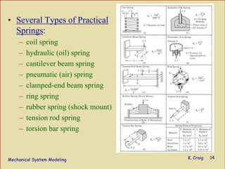
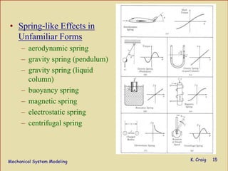
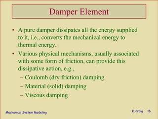
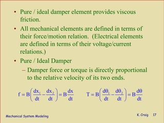
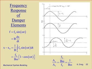
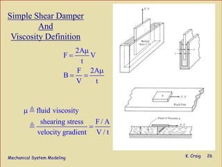
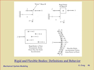
This document discusses modeling mechanical systems using three basic elements: springs, dampers, and masses. It describes the properties and dynamic responses of ideal spring and damper elements and provides examples of real-world springs and dampers. The document also discusses modeling nonlinear springs and damping effects in mechanical systems.
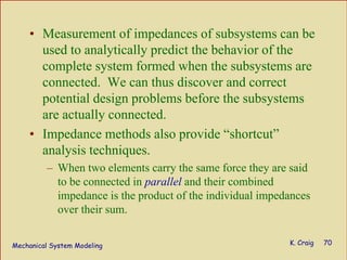
![Mechanical System Modeling K. Craig 85
Physical System
Physical Model
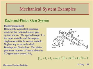
Problem Statement
A dynamic vibration absorber consists of
a mass and an elastic element that is
attached to another mass in order to
reduce its vibration. The figure is a
representation of a vibration absorber
attached to the cantilever support. For a
cantilever beam with a force at its end, k
= Ewh3/4L3 where L = beam length, w =
beam width, and h = beam thickness. (a)
Obtain the equation of motion for the
system. The force f is a specified force
acting on the mass m, and is due to the
rotating unbalance of the motor. The
displacements x and x2 are measured
from the static equilibrium positions
when f = 0. (b) Obtain the transfer
functions x/f and x2/f.
( )[ ]
( )[ ]
2
2 2
4 2
2 2 2 2 2
2 2
4 2
2 2 2 2 2
m D kx
F mm D m k k mk D kk
x k
F mm D m k k mk D kk
+
=
+ + + +
=
+ + + +
Dynamic Vibration Absorber](https://image.slidesharecdn.com/modelingofmechanicalsystems-141021131232-conversion-gate02/85/Modeling-of-mechanical_systems-85-320.jpg)