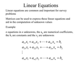
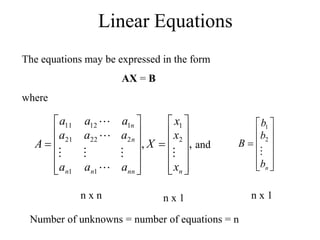
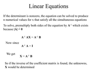
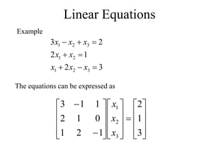
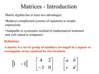
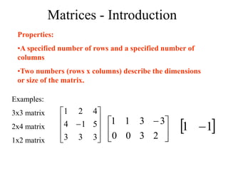
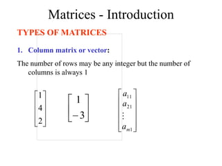
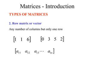
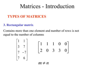
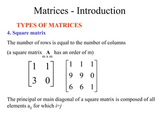
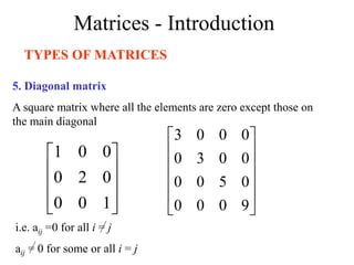
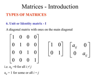
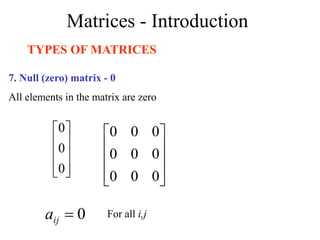
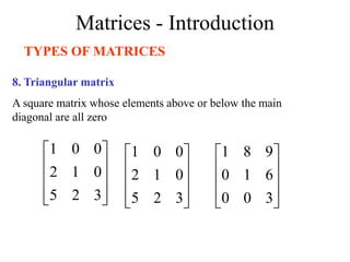
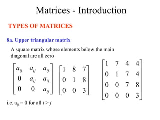
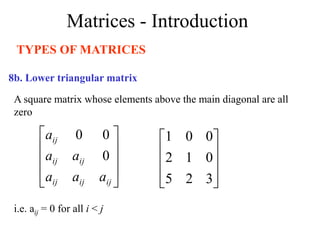
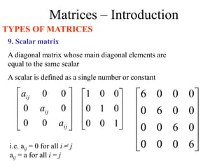
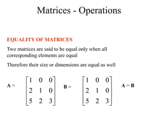
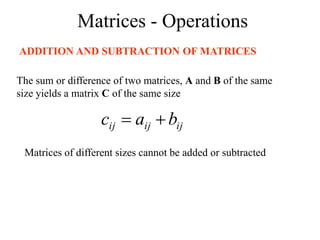
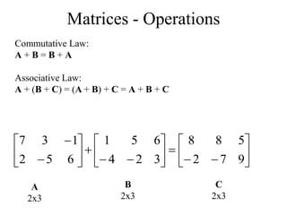
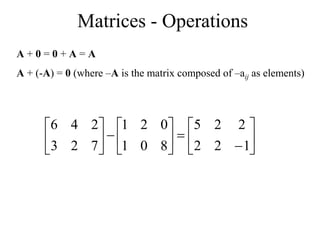
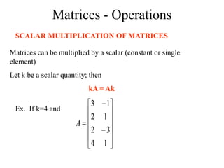
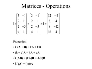
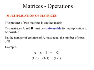
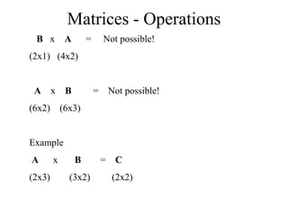
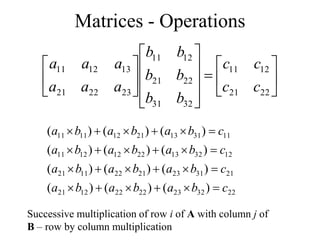
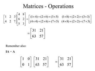
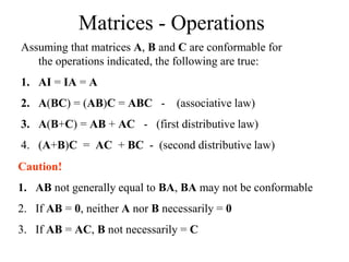
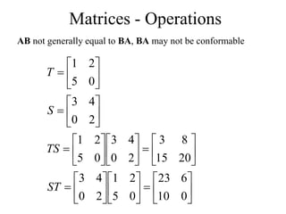
Matrices can be represented as arrays of numbers arranged in rows and columns. A matrix is defined by its dimensions (number of rows and columns). There are several types of matrices including square, rectangular, diagonal, identity, null, triangular, and scalar matrices. Operations on matrices include addition, subtraction, and multiplication. For matrices to be added or subtracted, they must be the same size. Matrices can be multiplied by a scalar value. Matrix multiplication results in another matrix, and the number of columns of the first matrix must equal the number of rows of the second matrix.

1. Matrices
Introduction

2. Matrices - Introduction
Matrix algebra has at least two advantages:
•Reduces complicated systems of equations to simple
expressions
•Adaptable to systematic method of mathematical treatment
and well suited to computers
Definition:
A matrix is a set or group of numbers arranged in a square or
rectangular array enclosed by two brackets
 
1
1  





 0
3
2
4






d
c
b
a

3. Matrices - Introduction
Properties:
•A specified number of rows and a specified number of
columns
•Two numbers (rows x columns) describe the dimensions
or size of the matrix.
Examples:
3x3 matrix
2x4 matrix
1x2 matrix 










3
3
3
5
1
4
4
2
1





 
2
3
3
3
0
1
0
1
 
1
1 

4. Matrices - Introduction
A matrix is denoted by a bold capital letter and the elements
within the matrix are denoted by lower case letters
e.g. matrix [A] with elements aij














mn
ij
m
m
n
ij
in
ij
a
a
a
a
a
a
a
a
a
a
a
a
2
1
2
22
21
12
11
...
...




i goes from 1 to m
j goes from 1 to n
Amxn=
mAn

5. Matrices - Introduction
TYPES OF MATRICES
1. Column matrix or vector:
The number of rows may be any integer but the number of
columns is always 1










2
4
1






3
1












1
21
11
m
a
a
a


6. Matrices - Introduction
TYPES OF MATRICES
2. Row matrix or vector
Any number of columns but only one row
 
6
1
1  
2
5
3
0
 
n
a
a
a
a 1
13
12
11 

7. Matrices - Introduction
TYPES OF MATRICES
3. Rectangular matrix
Contains more than one element and number of rows is not
equal to the number of columns













6
7
7
7
7
3
1
1






0
3
3
0
2
0
0
1
1
1
n
m 

8. Matrices - Introduction
TYPES OF MATRICES
4. Square matrix
The number of rows is equal to the number of columns
(a square matrix A has an order of m)






0
3
1
1










1
6
6
0
9
9
1
1
1
m x m
The principal or main diagonal of a square matrix is composed of all
elements aij for which i=j

9. Matrices - Introduction
TYPES OF MATRICES
5. Diagonal matrix
A square matrix where all the elements are zero except those on
the main diagonal










1
0
0
0
2
0
0
0
1












9
0
0
0
0
5
0
0
0
0
3
0
0
0
0
3
i.e. aij =0 for all i = j
aij = 0 for some or all i = j

10. Matrices - Introduction
TYPES OF MATRICES
6. Unit or Identity matrix - I
A diagonal matrix with ones on the main diagonal












1
0
0
0
0
1
0
0
0
0
1
0
0
0
0
1






1
0
0
1
i.e. aij =0 for all i = j
aij = 1 for some or all i = j






ij
ij
a
a
0
0

11. Matrices - Introduction
TYPES OF MATRICES
7. Null (zero) matrix - 0
All elements in the matrix are zero










0
0
0










0
0
0
0
0
0
0
0
0
0

ij
a For all i,j

12. Matrices - Introduction
TYPES OF MATRICES
8. Triangular matrix
A square matrix whose elements above or below the main
diagonal are all zero










3
2
5
0
1
2
0
0
1










3
2
5
0
1
2
0
0
1










3
0
0
6
1
0
9
8
1

13. Matrices - Introduction
TYPES OF MATRICES
8a. Upper triangular matrix
A square matrix whose elements below the main
diagonal are all zero
i.e. aij = 0 for all i > j










3
0
0
8
1
0
7
8
1












3
0
0
0
8
7
0
0
4
7
1
0
4
4
7
1










ij
ij
ij
ij
ij
ij
a
a
a
a
a
a
0
0
0

14. Matrices - Introduction
TYPES OF MATRICES
A square matrix whose elements above the main diagonal are all
zero
8b. Lower triangular matrix
i.e. aij = 0 for all i < j










3
2
5
0
1
2
0
0
1










ij
ij
ij
ij
ij
ij
a
a
a
a
a
a
0
0
0

15. Matrices – Introduction
TYPES OF MATRICES
9. Scalar matrix
A diagonal matrix whose main diagonal elements are
equal to the same scalar
A scalar is defined as a single number or constant










1
0
0
0
1
0
0
0
1












6
0
0
0
0
6
0
0
0
0
6
0
0
0
0
6
i.e. aij = 0 for all i = j
aij = a for all i = j










ij
ij
ij
a
a
a
0
0
0
0
0
0

16. Matrices
Matrix Operations

17. Matrices - Operations
EQUALITY OF MATRICES
Two matrices are said to be equal only when all
corresponding elements are equal
Therefore their size or dimensions are equal as well










3
2
5
0
1
2
0
0
1










3
2
5
0
1
2
0
0
1
A = B = A = B

18. Matrices - Operations
Some properties of equality:
•IIf A = B, then B = A for all A and B
•IIf A = B, and B = C, then A = C for all A, B and C










3
2
5
0
1
2
0
0
1
A = B =










33
32
31
23
22
21
13
12
11
b
b
b
b
b
b
b
b
b
If A = B then ij
ij b
a 

19. Matrices - Operations
ADDITION AND SUBTRACTION OF MATRICES
The sum or difference of two matrices, A and B of the same
size yields a matrix C of the same size
ij
ij
ij b
a
c 

Matrices of different sizes cannot be added or subtracted

20. Matrices - Operations
Commutative Law:
A + B = B + A
Associative Law:
A + (B + C) = (A + B) + C = A + B + C


























9
7
2
5
8
8
3
2
4
6
5
1
6
5
2
1
3
7
A
2x3
B
2x3
C
2x3

21. Matrices - Operations
A + 0 = 0 + A = A
A + (-A) = 0 (where –A is the matrix composed of –aij as elements)





















1
2
2
2
2
5
8
0
1
0
2
1
7
2
3
2
4
6

22. Matrices - Operations
SCALAR MULTIPLICATION OF MATRICES
Matrices can be multiplied by a scalar (constant or single
element)
Let k be a scalar quantity; then
kA = Ak
Ex. If k=4 and















1
4
3
2
1
2
1
3
A

23. Matrices - Operations














































4
16
12
8
4
8
4
12
4
1
4
3
2
1
2
1
3
1
4
3
2
1
2
1
3
4
Properties:
• k (A + B) = kA + kB
• (k + g)A = kA + gA
• k(AB) = (kA)B = A(k)B
• k(gA) = (kg)A

24. Matrices - Operations
MULTIPLICATION OF MATRICES
The product of two matrices is another matrix
Two matrices A and B must be conformable for multiplication to
be possible
i.e. the number of columns of A must equal the number of rows
of B
Example.
A x B = C
(1x3) (3x1) (1x1)

25. Matrices - Operations
B x A = Not possible!
(2x1) (4x2)
A x B = Not possible!
(6x2) (6x3)
Example
A x B = C
(2x3) (3x2) (2x2)

26. Matrices - Operations























22
21
12
11
32
31
22
21
12
11
23
22
21
13
12
11
c
c
c
c
b
b
b
b
b
b
a
a
a
a
a
a
22
32
23
22
22
12
21
21
31
23
21
22
11
21
12
32
13
22
12
12
11
11
31
13
21
12
11
11
)
(
)
(
)
(
)
(
)
(
)
(
)
(
)
(
)
(
)
(
)
(
)
(
c
b
a
b
a
b
a
c
b
a
b
a
b
a
c
b
a
b
a
b
a
c
b
a
b
a
b
a
























Successive multiplication of row i of A with column j of
B – row by column multiplication

27. Matrices - Operations











































)
3
7
(
)
2
2
(
)
8
4
(
)
5
7
(
)
6
2
(
)
4
4
(
)
3
3
(
)
2
2
(
)
8
1
(
)
5
3
(
)
6
2
(
)
4
1
(
3
5
2
6
8
4
7
2
4
3
2
1







57
63
21
31
Remember also:
IA = A






1
0
0
1






57
63
21
31







57
63
21
31

28. Matrices - Operations
Assuming that matrices A, B and C are conformable for
the operations indicated, the following are true:
1. AI = IA = A
2. A(BC) = (AB)C = ABC - (associative law)
3. A(B+C) = AB + AC - (first distributive law)
4. (A+B)C = AC + BC - (second distributive law)
Caution!
1. AB not generally equal to BA, BA may not be conformable
2. If AB = 0, neither A nor B necessarily = 0
3. If AB = AC, B not necessarily = C

29. Matrices - Operations
AB not generally equal to BA, BA may not be conformable






















































0
10
6
23
0
5
2
1
2
0
4
3
20
15
8
3
2
0
4
3
0
5
2
1
2
0
4
3
0
5
2
1
ST
TS
S
T

30. Matrices - Operations
If AB = 0, neither A nor B necessarily = 0





















0
0
0
0
3
2
3
2
0
0
1
1

31. Matrices - Operations
TRANSPOSE OF A MATRIX
If :








1
3
5
7
4
2
3
2 A
A
2x3












1
7
3
4
5
2
3
2
T
T
A
A
Then transpose of A, denoted AT is:
T
ji
ij a
a  For all i and j

32. Matrices - Operations
To transpose:
Interchange rows and columns
The dimensions of AT are the reverse of the dimensions of A








1
3
5
7
4
2
3
2 A
A












1
7
3
4
5
2
2
3
T
T
A
A
2 x 3
3 x 2

33. Matrices - Operations
Properties of transposed matrices:
1. (A+B)T = AT + BT
2. (AB)T = BT AT
3. (kA)T = kAT
4. (AT)T = A

34. Matrices - Operations
1. (A+B)T = AT + BT


























9
7
2
5
8
8
3
2
4
6
5
1
6
5
2
1
3
7












9
5
7
8
2
8






































9
5
7
8
2
8
3
6
2
5
4
1
6
1
5
3
2
7

35. Matrices - Operations
(AB)T = BT AT
 
   
8
2
3
0
2
1
0
1
2
1
1
8
2
8
2
2
1
1
3
2
0
0
1
1




































36. Matrices - Operations
SYMMETRIC MATRICES
A Square matrix is symmetric if it is equal to its
transpose:
A = AT














d
b
b
a
A
d
b
b
a
A
T

37. Matrices - Operations
When the original matrix is square, transposition does not
affect the elements of the main diagonal














d
b
c
a
A
d
c
b
a
A
T
The identity matrix, I, a diagonal matrix D, and a scalar matrix, K,
are equal to their transpose since the diagonal is unaffected.

38. Matrices - Operations
INVERSE OF A MATRIX
Consider a scalar k. The inverse is the reciprocal or division of 1
by the scalar.
Example:
k=7 the inverse of k or k-1 = 1/k = 1/7
Division of matrices is not defined since there may be AB = AC
while B = C
Instead matrix inversion is used.
The inverse of a square matrix, A, if it exists, is the unique matrix
A-1 where:
AA-1 = A-1 A = I

39. Matrices - Operations
Example:


















3
2
1
1
1
2
1
3
1
2
2
A
A
A










































1
0
0
1
3
2
1
1
1
2
1
3
1
0
0
1
1
2
1
3
3
2
1
1
Because:

40. Matrices - Operations
Properties of the inverse:
1
1
1
1
1
1
1
1
1
1
)
(
)
(
)
(
)
(
)
(













A
k
kA
A
A
A
A
A
B
AB
T
T
A square matrix that has an inverse is called a nonsingular matrix
A matrix that does not have an inverse is called a singular matrix
Square matrices have inverses except when the determinant is zero
When the determinant of a matrix is zero the matrix is singular

41. Matrices - Operations
DETERMINANT OF A MATRIX
To compute the inverse of a matrix, the determinant is required
Each square matrix A has a unit scalar value called the
determinant of A, denoted by det A or |A|
5
6
2
1
5
6
2
1








A
A
If
then

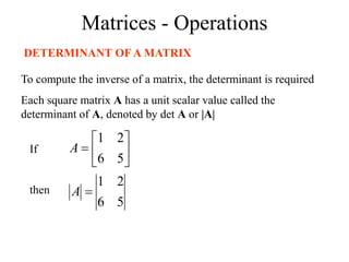
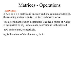
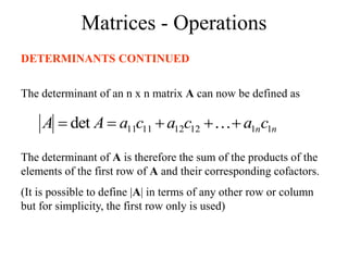
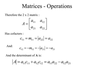
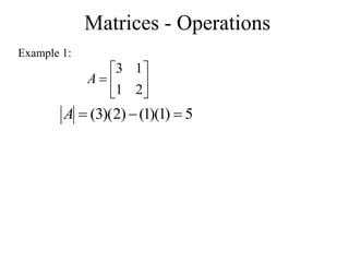
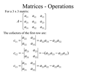
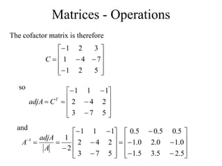
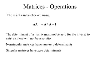
42. Matrices - Operations
If A = [A] is a single element (1x1), then the determinant is
defined as the value of the element
Then |A| =det A = a11
If A is (n x n), its determinant may be defined in terms of order
(n-1) or less.

43. Matrices - Operations
MINORS
If A is an n x n matrix and one row and one column are deleted,
the resulting matrix is an (n-1) x (n-1) submatrix of A.
The determinant of such a submatrix is called a minor of A and
is designated by mij , where i and j correspond to the deleted
row and column, respectively.
mij is the minor of the element aij in A.

44. Matrices - Operations











33
32
31
23
22
21
13
12
11
a
a
a
a
a
a
a
a
a
A
Each element in A has a minor
Delete first row and column from A .
The determinant of the remaining 2 x 2 submatrix is the minor
of a11
eg.
33
32
23
22
11
a
a
a
a
m 

45. Matrices - Operations
Therefore the minor of a12 is:
And the minor for a13 is:
33
31
23
21
12
a
a
a
a
m 
32
31
22
21
13
a
a
a
a
m 

46. Matrices - Operations
COFACTORS
The cofactor Cij of an element aij is defined as:
ij
j
i
ij m
C 

 )
1
(
When the sum of a row number i and column j is even, cij = mij and
when i+j is odd, cij =-mij
13
13
3
1
13
12
12
2
1
12
11
11
1
1
11
)
1
(
)
3
,
1
(
)
1
(
)
2
,
1
(
)
1
(
)
1
,
1
(
m
m
j
i
c
m
m
j
i
c
m
m
j
i
c






















47. Matrices - Operations
DETERMINANTS CONTINUED
The determinant of an n x n matrix A can now be defined as
n
nc
a
c
a
c
a
A
A 1
1
12
12
11
11
det 



 
The determinant of A is therefore the sum of the products of the
elements of the first row of A and their corresponding cofactors.
(It is possible to define |A| in terms of any other row or column
but for simplicity, the first row only is used)

48. Matrices - Operations
Therefore the 2 x 2 matrix :







22
21
12
11
a
a
a
a
A
Has cofactors :
22
22
11
11 a
a
m
c 


And:
21
21
12
12 a
a
m
c 





And the determinant of A is:
21
12
22
11
12
12
11
11 a
a
a
a
c
a
c
a
A 




49. Matrices - Operations
Example 1:







2
1
1
3
A
5
)
1
)(
1
(
)
2
)(
3
( 


A

50. Matrices - Operations
For a 3 x 3 matrix:











33
32
31
23
22
21
13
12
11
a
a
a
a
a
a
a
a
a
A
The cofactors of the first row are:
31
22
32
21
32
31
22
21
13
31
23
33
21
33
31
23
21
12
32
23
33
22
33
32
23
22
11
)
(
a
a
a
a
a
a
a
a
c
a
a
a
a
a
a
a
a
c
a
a
a
a
a
a
a
a
c












51. Matrices - Operations
The determinant of a matrix A is:
21
12
22
11
12
12
11
11 a
a
a
a
c
a
c
a
A 



Which by substituting for the cofactors in this case is:
)
(
)
(
)
( 31
22
32
21
13
31
23
33
21
12
32
23
33
22
11 a
a
a
a
a
a
a
a
a
a
a
a
a
a
a
A 






52. Matrices - Operations
Example 2:












1
0
1
3
2
0
1
0
1
A
4
)
2
0
)(
1
(
)
3
0
)(
0
(
)
0
2
)(
1
( 






A
)
(
)
(
)
( 31
22
32
21
13
31
23
33
21
12
32
23
33
22
11 a
a
a
a
a
a
a
a
a
a
a
a
a
a
a
A 






53. Matrices - Operations
ADJOINT MATRICES
A cofactor matrix C of a matrix A is the square matrix of the same
order as A in which each element aij is replaced by its cofactor cij .
Example:








4
3
2
1
A








1
2
3
4
C
If
The cofactor C of A is

54. Matrices - Operations
The adjoint matrix of A, denoted by adj A, is the transpose of its
cofactor matrix
T
C
adjA
It can be shown that:
A(adj A) = (adjA) A = |A| I
Example:





 














1
3
2
4
10
)
3
)(
2
(
)
4
)(
1
(
4
3
2
1
T
C
adjA
A
A

55. Matrices - Operations
I
adjA
A 10
10
0
0
10
1
3
2
4
4
3
2
1
)
( 












 








I
A
adjA 10
10
0
0
10
4
3
2
1
1
3
2
4
)
( 



















 


56. Matrices - Operations
USING THE ADJOINT MATRIX IN MATRIX INVERSION
A
adjA
A 
1
Since
AA-1 = A-1 A = I
and
A(adj A) = (adjA) A = |A| I
then

57. Matrices - Operations
Example





 






 


1
.
0
3
.
0
2
.
0
4
.
0
1
3
2
4
10
1
1
A






 4
3
2
1
A =
To check AA-1 = A-1 A = I
I
A
A
I
AA




















 














 










1
0
0
1
4
3
2
1
1
.
0
3
.
0
2
.
0
4
.
0
1
0
0
1
1
.
0
3
.
0
2
.
0
4
.
0
4
3
2
1
1
1

58. Matrices - Operations
Example 2













1
2
1
0
1
2
1
1
3
A
|A| = (3)(-1-0)-(-1)(-2-0)+(1)(4-1) = -2
),
1
(
),
1
(
),
1
(
31
21
11









c
c
c
The determinant of A is
The elements of the cofactor matrix are
),
2
(
),
4
(
),
2
(
32
22
12









c
c
c
),
5
(
),
7
(
),
3
(
33
23
13






c
c
c

59. Matrices - Operations















5
2
1
7
4
1
3
2
1
C
The cofactor matrix is therefore
so
















5
7
3
2
4
2
1
1
1
T
C
adjA
and


































5
.
2
5
.
3
5
.
1
0
.
1
0
.
2
0
.
1
5
.
0
5
.
0
5
.
0
5
7
3
2
4
2
1
1
1
2
1
1
A
adjA
A

60. Matrices - Operations
The result can be checked using
AA-1 = A-1 A = I
The determinant of a matrix must not be zero for the inverse to
exist as there will not be a solution
Nonsingular matrices have non-zero determinants
Singular matrices have zero determinants

61. Matrix Inversion
Simple 2 x 2 case

62. Simple 2 x 2 case
Let







d
c
b
a
A
and








z
y
x
w
A 1
Since it is known that
A A-1 = I
then



















1
0
0
1
z
y
x
w
d
c
b
a

63. Simple 2 x 2 case
Multiplying gives
1
0
0
1








dz
cx
dy
cw
bz
ax
by
aw
bc
ad
A 

It can simply be shown that

64. Simple 2 x 2 case
thus
A
d
bc
da
d
w
d
cw
b
aw
d
cw
y
b
aw
y










1
1

65. Simple 2 x 2 case
A
b
bc
da
b
x
d
cx
b
ax
d
cx
z
b
ax
z












1
1

66. Simple 2 x 2 case
A
c
cb
ad
c
y
c
dy
a
by
c
dy
w
a
by
w












1
1

67. Simple 2 x 2 case
A
a
bc
ad
a
z
c
dz
a
bz
c
dz
x
a
bz
x










1
1

68. Simple 2 x 2 case
So that for a 2 x 2 matrix the inverse can be constructed
in a simple fashion as





















 a
c
b
d
A
A
a
A
c
A
b
A
d
1
•Exchange elements of main diagonal
•Change sign in elements off main diagonal
•Divide resulting matrix by the determinant









z
y
x
w
A 1

69. Simple 2 x 2 case
Example



























2
.
0
4
.
0
3
.
0
1
.
0
2
4
3
1
10
1
1
4
3
2
1
A
A
Check inverse
A-1 A=I
I























1
0
0
1
1
4
3
2
2
4
3
1
10
1

70. Matrices and Linear Equations
Linear Equations

71. Linear Equations
Linear equations are common and important for survey
problems
Matrices can be used to express these linear equations and
aid in the computation of unknown values
Example
n equations in n unknowns, the aij are numerical coefficients,
the bi are constants and the xj are unknowns
n
n
nn
n
n
n
n
n
n
b
x
a
x
a
x
a
b
x
a
x
a
x
a
b
x
a
x
a
x
a
















2
2
1
1
2
2
2
22
1
21
1
1
2
12
1
11

72. Linear Equations
The equations may be expressed in the form
AX = B
where
,
, 2
1
1
1
2
22
21
1
12
11


























n
nn
n
n
n
n
x
x
x
X
a
a
a
a
a
a
a
a
a
A







and













n
b
b
b
B

2
1
n x n n x 1 n x 1
Number of unknowns = number of equations = n

73. Linear Equations
If the determinant is nonzero, the equation can be solved to produce
n numerical values for x that satisfy all the simultaneous equations
To solve, premultiply both sides of the equation by A-1 which exists
because |A| = 0
A-1 AX = A-1 B
Now since
A-1 A = I
We get
X = A-1 B
So if the inverse of the coefficient matrix is found, the unknowns,
X would be determined

74. Linear Equations
Example
3
2
1
2
2
3
3
2
1
2
1
3
2
1








x
x
x
x
x
x
x
x
The equations can be expressed as

































3
1
2
1
2
1
0
1
2
1
1
3
3
2
1
x
x
x

75. Linear Equations
When A-1 is computed the equation becomes






































 
7
3
2
3
1
2
5
.
2
5
.
3
5
.
1
0
.
1
0
.
2
0
.
1
5
.
0
5
.
0
5
.
0
1
B
A
X
Therefore
7
,
3
,
2
3
2
1





x
x
x

76. Linear Equations
The values for the unknowns should be checked by substitution
back into the initial equations
3
2
1
2
2
3
3
2
1
2
1
3
2
1








x
x
x
x
x
x
x
x
3
)
7
(
)
3
(
2
)
2
(
1
)
3
(
)
2
(
2
2
)
7
(
)
3
(
)
2
(
3
















7
,
3
,
2
3
2
1





x
x
x