The document provides MATLAB programs for signal processing tasks including representation of basic signals, linear and circular convolution, overlap save and overlap add methods for convolution, and crosscorrelation and autocorrelation. It includes MATLAB code to generate unit impulse, step, ramp, exponential, sine and cosine signals. Code is also provided to compute linear convolution, circular convolution with and without zero padding, and implement overlap save and overlap add methods for convolution of sequences. Crosscorrelation and autocorrelation code is given as well.
![MATLAB Programs
Chapter 16
16.1 INTRODUCTION
MATLAB stands for MATrix LABoratory. It is a technical computing environment
for high performance numeric computation and visualisation. It integrates numerical
analysis, matrix computation, signal processing and graphics in an easy-to-use
environment, where problems and solutions are expressed just as they are written
mathematically, without traditional programming. MATLAB allows us to express
the entire algorithm in a few dozen lines, to compute the solution with great accuracy
in a few minutes on a computer, and to readily manipulate a three-dimensional
display of the result in colour.
MATLAB is an interactive system whose basic data element is a matrix that
does not require dimensioning. It enables us to solve many numerical problems in a
fraction of the time that it would take to write a program and execute in a language
such as FORTRAN, BASIC, or C. It also features a family of application specific
solutions, called toolboxes. Areas in which toolboxes are available include signal
processing, image processing, control systems design, dynamic systems simulation,
systems identification, neural networks, wavelength communication and others.
It can handle linear, non-linear, continuous-time, discrete-time, multivariable and
multirate systems. This chapter gives simple programs to solve specific problems
that are included in the previous chapters. All these MATLAB programs have been
tested under version 7.1 of MATLAB and version 6.12 of the signal processing
toolbox.
16.2 REPRESENTATION OF BASIC SIGNALS
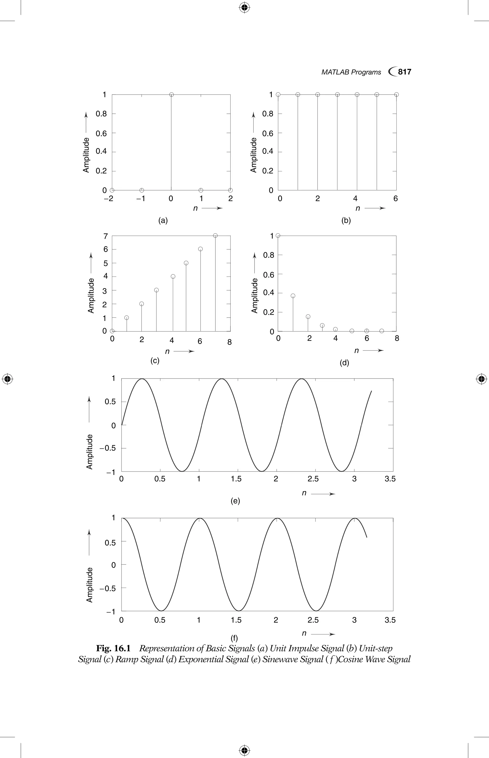
MATLAB programs for the generation of unit impulse, unit step, ramp, exponential,
sinusoidal and cosine sequences are as follows.
% Program for the generation of unit impulse signal
clc;clear all;close all;
t522:1:2;
y5[zeros(1,2),ones(1,1),zeros(1,2)];subplot(2,2,1);stem(t,y);](https://image.slidesharecdn.com/matlabprograms-150130053105-conversion-gate01/75/Matlab-programs-1-2048.jpg)
![816 Digital Signal Processing
ylabel(‘Amplitude --.’);
xlabel(‘(a) n --.’);
% Program for the generation of unit step sequence [u(n)2 u(n 2 N]
n5input(‘enter the N value’);
t50:1:n21;
y15ones(1,n);subplot(2,2,2);
stem(t,y1);ylabel(‘Amplitude --.’);
xlabel(‘(b) n --.’);
% Program for the generation of ramp sequence
n15input(‘enter the length of ramp sequence’);
t50:n1;
subplot(2,2,3);stem(t,t);ylabel(‘Amplitude --.’);
xlabel(‘(c) n --.’);
% Program for the generation of exponential sequence
n25input(‘enter the length of exponential sequence’);
t50:n2;
a5input(‘Enter the ‘a’ value’);
y25exp(a*t);subplot(2,2,4);
stem(t,y2);ylabel(‘Amplitude --.’);
xlabel(‘(d) n --.’);
% Program for the generation of sine sequence
t50:.01:pi;
y5sin(2*pi*t);figure(2);
subplot(2,1,1);plot(t,y);ylabel(‘Amplitude --.’);
xlabel(‘(a) n --.’);
% Program for the generation of cosine sequence
t50:.01:pi;
y5cos(2*pi*t);
subplot(2,1,2);plot(t,y);ylabel(‘Amplitude --.’);
xlabel(‘(b) n --.’);
As an example,
enter the N value 7
enter the length of ramp sequence 7
enter the length of exponential sequence 7
enter the a value 1
Using the above MATLAB programs, we can obtain the waveforms of the unit
impulse signal, unit step signal, ramp signal, exponential signal, sine wave signal and
cosine wave signal as shown in Fig. 16.1.](https://image.slidesharecdn.com/matlabprograms-150130053105-conversion-gate01/75/Matlab-programs-2-2048.jpg)
![818 Digital Signal Processing
16.3 DISCRETE CONVOLUTION
16.3.1 Linear Convolution
Algorithm
1. Get two signals x(m)and h(p)in matrix form
2. The convolved signal is denoted as y(n)
3. y(n)is given by the formula
y(n) 5 [ ( ) ( )]x k h n k
k
−
=−∞
∞
∑ where n50 to m 1 p 2 1
4. Stop
% Program for linear convolution of the sequence x5[1, 2] and h5[1, 2, 4]
clc;
clear all;
close all;
x5input(‘enter the 1st sequence’);
h5input(‘enter the 2nd sequence’);
y5conv(x,h);
figure;subplot(3,1,1);
stem(x);ylabel(‘Amplitude --.’);
xlabel(‘(a) n --.’);
subplot(3,1,2);
stem(h);ylabel(‘Amplitude --.’);
xlabel(‘(b) n --.’);
subplot(3,1,3);
stem(y);ylabel(‘Amplitude --.’);
xlabel(‘(c) n --.’);
disp(‘The resultant signal is’);y
As an example,
enter the 1st sequence [1 2]
enter the 2nd sequence [1 2 4]
The resultant signal is
y51 4 8 8
Figure 16.2 shows the discrete input signals x(n)and h(n)and the convolved output
signal y(n).
Fig. 16.2 (Contd.)
AmplitudeAmplitude
n
n
0
0
0.5
1
1
1
1.1
1.2
1.2
1.4
1.3
1.6
1.4
1.8
1.5
2
(a)
(b)
1.6
2.2
1.7
2.4
1.8
2.6
1.9
2.8
2
3
1
2
1.5
3
2
4](https://image.slidesharecdn.com/matlabprograms-150130053105-conversion-gate01/75/Matlab-programs-4-2048.jpg)
![MATLAB Programs 819
16.3.2 Circular Convolution
% Program for Computing Circular Convolution
clc;
clear;
a = input(‘enter the sequence x(n) = ’);
b = input(‘enter the sequence h(n) = ’);
n1=length(a);
n2=length(b);
N=max(n1,n2);
x = [a zeros(1,(N-n1))];
for i = 1:N
k = i;
for j = 1:n2
H(i,j)=x(k)* b(j);
k = k-1;
if (k == 0)
k = N;
end
end
end
y=zeros(1,N);
M=H’;
for j = 1:N
for i = 1:n2
y(j)=M(i,j)+y(j);
end
end
disp(‘The output sequence is y(n)= ‘);
disp(y);
Fig. 16.2 Discrete Linear Convolution
AmplitudeAmplitudeAmplitude
n
n
n
0
0
0
0.5
1
2
1
1
1
1.1
1.2
1.2
1.4
1.5
1.3
1.6
1.4
1.8
1.5
2
2
(a)
(b)
(c)
1.6
2.2
2.5
1.7
2.4
3
1.8
2.6
3.5
1.9
2.8
2
3
4
1
2
4
1.5
3
6
2
4
8
AmplitudeAmplitudeAmplitude
n
n
n
0
0
0
0.5
1
2
1
1
1
1.1
1.2
1.2
1.4
1.5
1.3
1.6
1.4
1.8
1.5
2
2
(a)
(b)
(c)
1.6
2.2
2.5
1.7
2.4
3
1.8
2.6
3.5
1.9
2.8
2
3
4
1
2
4
1.5
3
6
2
4
8](https://image.slidesharecdn.com/matlabprograms-150130053105-conversion-gate01/75/Matlab-programs-5-2048.jpg)
![820 Digital Signal Processing
stem(y);
title(‘Circular Convolution’);
xlabel(‘n’);
ylabel(‚y(n)‘);
As an Example,
enter the sequence x(n) = [1 2 4]
enter the sequence h(n) = [1 2]
The output sequence is y(n)= 9 4 8
% Program for Computing Circular Convolution with zero padding
clc;
close all;
clear all;
g5input(‘enter the first sequence’);
h5input(‘enter the 2nd sequence’);
N15length(g);
N25length(h);
N5max(N1,N2);
N35N12N2;
%Loop for getting equal length sequence
if(N350)
h5[h,zeros(1,N3)];
else
g5[g,zeros(1,2N3)];
end
%computation of circular convolved sequence
for n51:N,
y(n)50;
for i51:N,
j5n2i11;
if(j550)
j5N1j;
end
y(n)5y(n)1g(i)*h(j);
end
end
disp(‘The resultant signal is’);y
As an example,
enter the first sequence [1 2 4]
enter the 2nd sequence [1 2]
The resultant signal is y51 4 8 8
16.3.3 Overlap Save Method and Overlap Add method
% Program for computing Block Convolution using Overlap Save
Method
Overlap Save Method
x=input(‘Enter the sequence x(n) = ’);](https://image.slidesharecdn.com/matlabprograms-150130053105-conversion-gate01/75/Matlab-programs-6-2048.jpg)
![MATLAB Programs 821
h=input(‘Enter the sequence h(n) = ’);
n1=length(x);
n2=length(h);
N=n1+n2-1;
h1=[h zeros(1,N-n1)];
n3=length(h1);
y=zeros(1,N);
x1=[zeros(1,n3-n2) x zeros(1,n3)];
H=fft(h1);
for i=1:n2:N
y1=x1(i:i+(2*(n3-n2)));
y2=fft(y1);
y3=y2.*H;
y4=round(ifft(y3));
y(i:(i+n3-n2))=y4(n2:n3);
end
disp(‘The output sequence y(n)=’);
disp(y(1:N));
stem(y(1:N));
title(‘Overlap Save Method’);
xlabel(‘n’);
ylabel(‘y(n)’);
Enter the sequence x(n) = [1 2 -1 2 3 -2 -3 -1 1 1 2 -1]
Enter the sequence h(n) = [1 2 3 -1]
The output sequence y(n) = 1 4 6 5 2 11 0 -16 -8 3 8 5 3 -5 1
%Program for computing Block Convolution using Overlap Add
Method
x=input(‘Enter the sequence x(n) = ’);
h=input(‘Enter the sequence h(n) = ’);
n1=length(x);
n2=length(h);
N=n1+n2-1;
y=zeros(1,N);
h1=[h zeros(1,n2-1)];
n3=length(h1);
y=zeros(1,N+n3-n2);
H=fft(h1);
for i=1:n2:n1
if i<=(n1+n2-1)
x1=[x(i:i+n3-n2) zeros(1,n3-n2)];
else
x1=[x(i:n1) zeros(1,n3-n2)];
end
x2=fft(x1);
x3=x2.*H;
x4=round(ifft(x3));
if (i==1)](https://image.slidesharecdn.com/matlabprograms-150130053105-conversion-gate01/75/Matlab-programs-7-2048.jpg)
![822 Digital Signal Processing
y(1:n3)=x4(1:n3);
else
y(i:i+n3-1)=y(i:i+n3-1)+x4(1:n3);
end
end
disp(‘The output sequence y(n)=’);
disp(y(1:N));
stem((y(1:N));
title(‘Overlap Add Method’);
xlabel(‘n’);
ylabel(‘y(n)’);
As an Example,
Enter the sequence x(n) = [1 2 -1 2 3 -2 -3 -1 1 1 2 -1]
Enter the sequence h(n) = [1 2 3 -1]
The output sequence
y(n) = 1 4 6 5 2 11 0 -16 -8 3 8 5 3 -5 1
16.4 DISCRETE CORRELATION
16.4.1 Crosscorrelation
Algorithm
1. Get two signals x(m)and h(p)in matrix form
2. The correlated signal is denoted as y(n)
3. y(n)is given by the formula
y(n) 5 [ ( ) ( )]x k h k n
k
−
=−∞
∞
∑
where n52 [max (m, p)2 1] to [max (m, p)2 1]
4. Stop
% Program for computing cross-correlation of the sequences
x5[1, 2, 3, 4] and h5[4, 3, 2, 1]
clc;
clear all;
close all;
x5input(‘enter the 1st sequence’);
h5input(‘enter the 2nd sequence’);
y5xcorr(x,h);
figure;subplot(3,1,1);
stem(x);ylabel(‘Amplitude --.’);
xlabel(‘(a) n --.’);
subplot(3,1,2);
stem(h);ylabel(‘Amplitude --.’);
xlabel(‘(b) n --.’);
subplot(3,1,3);
stem(fliplr(y));ylabel(‘Amplitude --.’);](https://image.slidesharecdn.com/matlabprograms-150130053105-conversion-gate01/75/Matlab-programs-8-2048.jpg)
![MATLAB Programs 823
xlabel(‘(c) n --.’);
disp(‘The resultant signal is’);fliplr(y)
As an example,
enter the 1st sequence [1 2 3 4]
enter the 2nd sequence [4 3 2 1]
The resultant signal is
y51.0000 4.0000 10.0000 20.
↑
0000 25.0000 24.0000 16.0000
Figure 16.3 shows the discrete input signals x(n)and h(n)and the cross-correlated
output signal y(n).
AmplitudeAmplitudeAmplitude
n
n
n
0
0
1
1
1
1
1
1.5
1.5
2
2
2
3
3
3
5
2.5
2.5
4
(a)
(b)
(c)
3.5
3.5
6
4
4
7
2
2
3
3
4
4
30
20
10
0
Fig. 16.3 Discrete Cross-correlation
16.4.2 Autocorrelation
Algorithm
1. Get the signal x(n)of length N in matrix form
2. The correlated signal is denoted as y(n)
3. y(n)is given by the formula
y(n) 5 [ ( ) ( )]x k x k n
k
−
=−∞
∞
∑
where n52(N 2 1) to (N 2 1)](https://image.slidesharecdn.com/matlabprograms-150130053105-conversion-gate01/75/Matlab-programs-9-2048.jpg)
![824 Digital Signal Processing
% Program for computing autocorrelation function
x5input(‘enter the sequence’);
y5xcorr(x,x);
figure;subplot(2,1,1);
stem(x);ylabel(‘Amplitude --.’);
xlabel(‘(a) n --.’);
subplot(2,1,2);
stem(fliplr(y));ylabel(‘Amplitude --.’);
xlabel(‘(a) n --.’);
disp(‘The resultant signal is’);fliplr(y)
As an example,
enter the sequence [1 2 3 4]
The resultant signal is
y54 11 20
↑
30 20 11 4
Figure 16.4 shows the discrete input signal x(n)and its auto-correlated output
signal y(n).
( )
AmplitudeAmplitude
n
n
0
1
1
1
1.5
2
2
3
3
(a)
5
2.5
4
(b) y (n)
3.5
6
4
7
2
3
4
0
5
10
15
20
25
30
Fig. 16.4 Discrete Auto-correlation
16.5 STABILITY TEST
% Program for stability test
clc;clear all;close all;
b5input(‘enter the denominator coefficients of the
filter’);
k5poly2rc(b);
knew5fliplr(k);
s5all(abs(knew)1);
if(s55 1)
disp(‘“Stable system”’);](https://image.slidesharecdn.com/matlabprograms-150130053105-conversion-gate01/75/Matlab-programs-10-2048.jpg)
![MATLAB Programs 825
else
disp(‘“Non-stable system”’);
end
As an example,
enter the denominator coefficients of the filter [1 21 .5]
“Stable system”
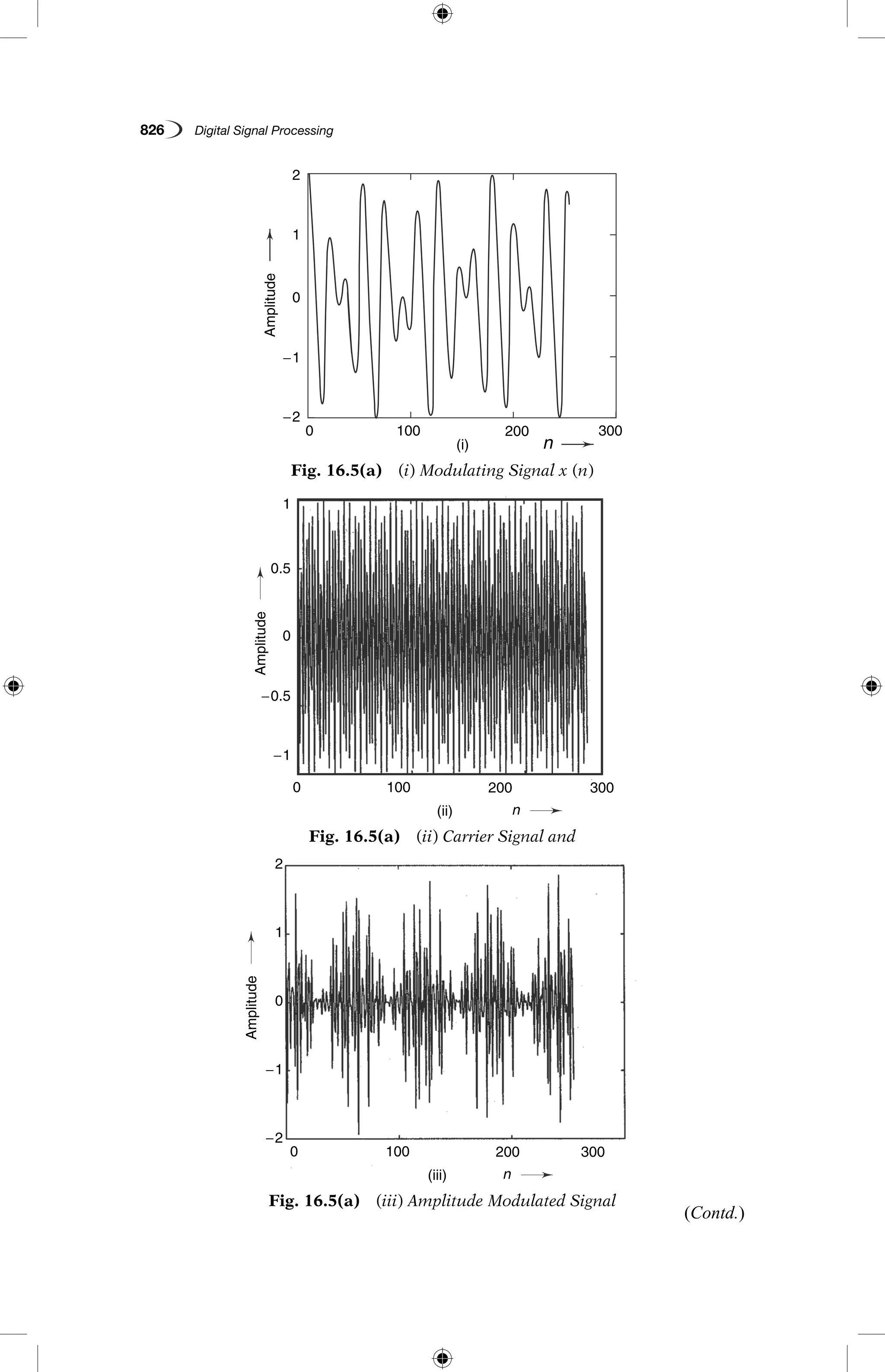
16.6 SAMPLING THEOREM
The sampling theorem can be understood well with the following example.
Example 16.1 Frequency analysis of the amplitude modulated discrete-time
signal
x(n)5cos 2 pf1
n 1 cos 2pf2
n
where f1
1
128
= and f2
5
128
= modulates the amplitude-modulated signal is
xc
(n)5cos 2p fc
n
where fc
550/128. The resulting amplitude-modulated signal is
xam
(n)5x(n) cos 2p fc
n
Using MATLAB program,
(a) sketch the signals x(n), xc
(n) and xam
(n), 0 # n # 255
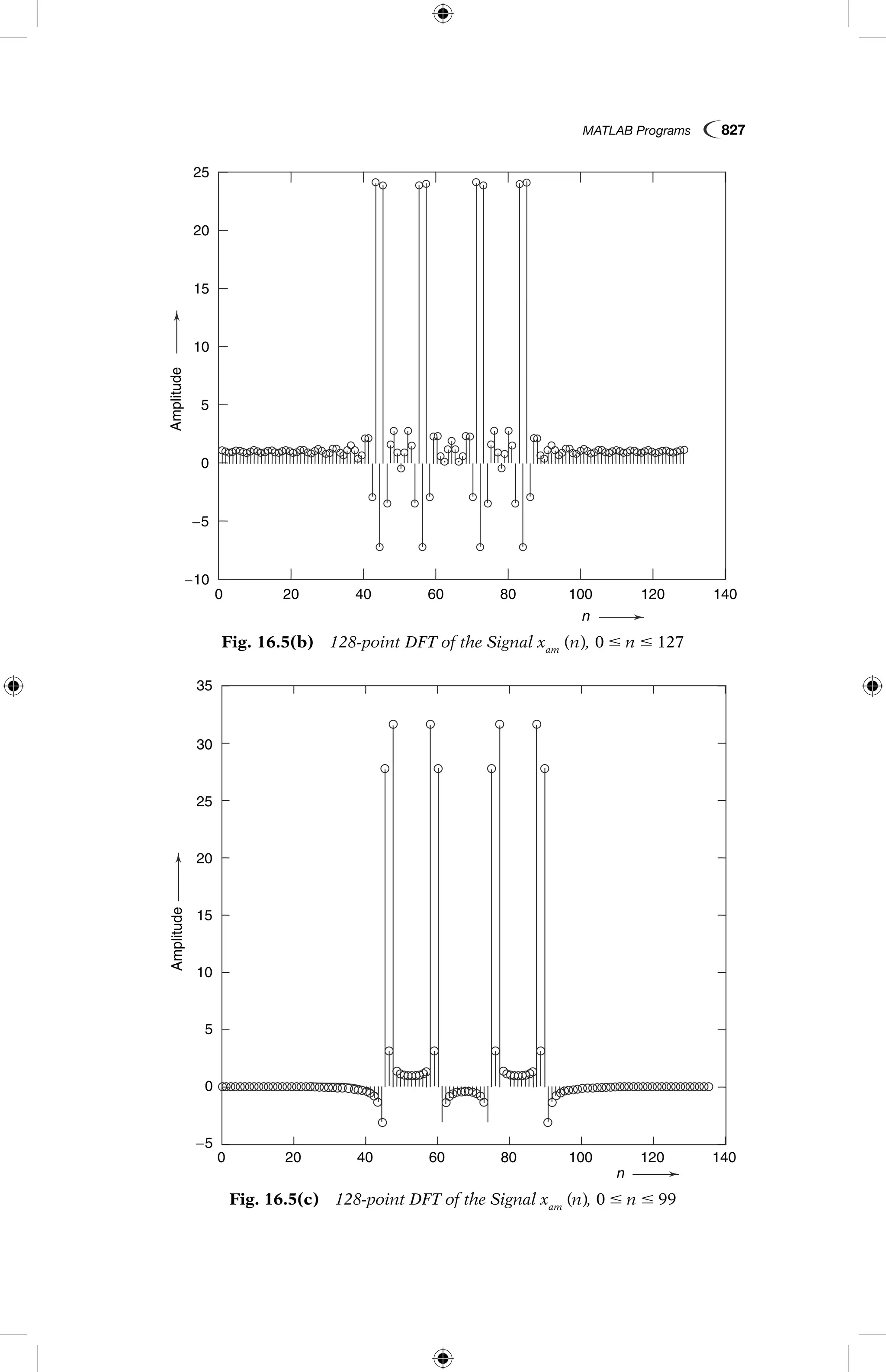
(b) compute and sketch the 128-point DFT of the signal xam
(n), 0 # n # 127
(c) compute and sketch the 128-point DFT of the signal xam
(n), 0 # n # 99
Solution
% Program
Solution for Section (a)
clc;close all;clear all;
f151/128;f255/128;n50:255;fc550/128;
x5cos(2*pi*f1*n)1cos(2*pi*f2*n);
xa5cos(2*pi*fc*n);
xamp5x.*xa;
subplot(2,2,1);plot(n,x);title(‘x(n)’);
xlabel(‘n --.’);ylabel(‘amplitude’);
subplot(2,2,2);plot(n,xc);title(‘xa(n)’);
xlabel(‘n --.’);ylabel(‘amplitude’);
subplot(2,2,3);plot(n,xamp);
xlabel(‘n --.’);ylabel(‘amplitude’);
%128 point DFT computation2solution for Section (b)
n50:127;figure;n15128;
f151/128;f255/128;fc550/128;
x5cos(2*pi*f1*n)1cos(2*pi*f2*n);
xc5cos(2*pi*fc*n);
xa5cos(2*pi*fc*n);
(Contd.)](https://image.slidesharecdn.com/matlabprograms-150130053105-conversion-gate01/75/Matlab-programs-11-2048.jpg)
![828 Digital Signal Processing
xamp5x.*xa;xam5fft(xamp,n1);
stem(n,xam);title(‘xamp(n)’);xlabel(‘n --.’);
ylabel(‘amplitude’);
%128 point DFT computation2solution for Section (c)
n50:99;figure;n250:n121;
f151/128;f255/128;fc550/128;
x5cos(2*pi*f1*n)1cos(2*pi*f2*n);
xc5cos(2*pi*fc*n);
xa5cos(2*pi*fc*n);
xamp5x.*xa;
for i51:100,
xamp1(i)5xamp(i);
end
xam5fft(xamp1,n1);
s t e m ( n 2 , x a m ) ; t i t l e ( ‘ x a m p ( n ) ’ ) ; x l a b e l ( ‘ n
--.’);ylabel(‘amplitude’);
(a)Modulated signal x(n), carrier signal xa
(n) and amplitude modulated signal
xam
(n) are shown in Fig. 16.5(a). Fig. 16.5 (b) shows the 128-point DFT of the
signal xam
(n) for 0 # n # 127 and Fig. 16.5 (c) shows the 128-point DFT of the
signal xam
(n), 0 # n # 99.
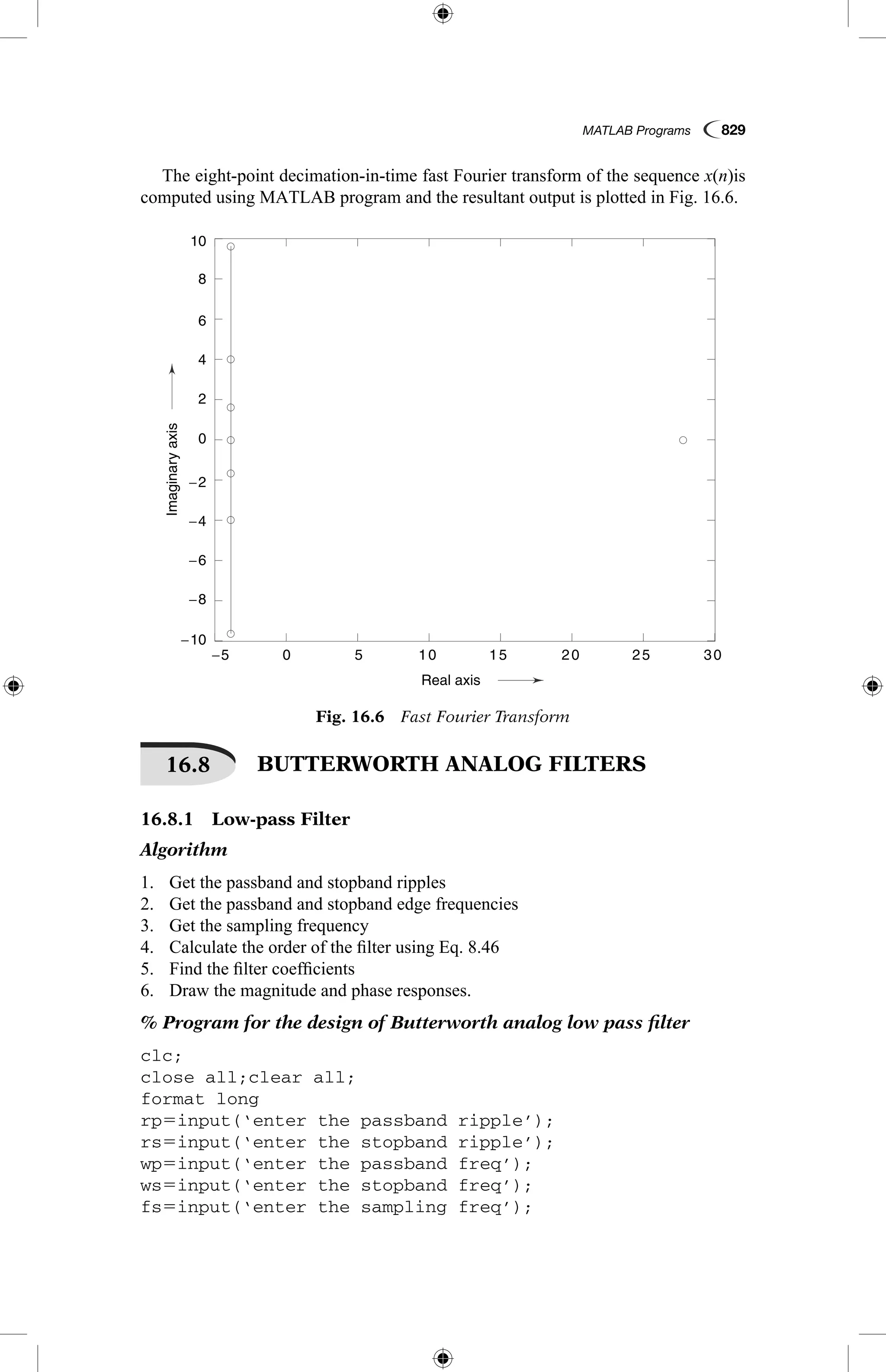
16.7 FAST FOURIER TRANSFORM
Algorithm
1. Get the signal x(n)of length N in matrix form
2. Get the N value
3. The transformed signal is denoted as
x k x n e k N
j
N
nk
n
N
( ) ( ) for= ≤ ≤ −
−
=
−
∑
2
0
1
0 1
p
% Program for computing discrete Fourier transform
clc;close all;clear all;
x5input(‘enter the sequence’);
n5input(‘enter the length of fft’);
X(k)5fft(x,n);
stem(y);ylabel(‘Imaginary axis --.’);
xlabel(‘Real axis --.’);
X(k)
As an example,
enter the sequence [0 1 2 3 4 5 6 7]
enter the length of fft 8
X(k)5
Columns 1 through 4
28.0000 24.000019.6569i 24.0000 14.0000i 24.0000
1 1.6569i
Columns 5 through 8
24.0000 24.0000 21.6569i 24.0000 24.0000i 24.0000
29.6569i](https://image.slidesharecdn.com/matlabprograms-150130053105-conversion-gate01/75/Matlab-programs-14-2048.jpg)
![830 Digital Signal Processing
w152*wp/fs;w252*ws/fs;
[n,wn]5buttord(w1,w2,rp,rs,’s’);
[z,p,k]5butter(n,wn);
[b,a]5zp2tf(z,p,k);
[b,a]5butter(n,wn,’s’);
w50:.01:pi;
[h,om]5freqs(b,a,w);
m520*log10(abs(h));
an5angle(h);
subplot(2,1,1);plot(om/pi,m);
ylabel(‘Gain in dB --.’);xlabel(‘(a) Normalised
frequency --.’);
subplot(2,1,2);plot(om/pi,an);
xlabel(‘(b) Normalised frequency --.’);
ylabel(‘Phase in radians --.’);
As an example,
enter the passband ripple 0.15
enter the stopband ripple 60
enter the passband freq 1500
enter the stopband freq 3000
enter the stopband freq 7000
The amplitude and phase responses of the Butterworth low-pass analog filter are
shown in Fig. 16.7.
Fig. 16.7 Butterworth Low-pass Analog Filter
(a) Amplitude Response and (b) Phase Response
0.1
0.1
−250
−200
−150
−4
−2
2
4
0
−100
−50
50
GainindB
0
0.2
0.2
0.3
0.3
0.4
0.4
(a)
(b)
Normalised frequency
Normalised frequency
0.5
0.5
0.6
0.6
0.7
0.7
0.8
0.8
0.9
0.9
1
1
0
0
Phaseinradians
0.1
0.1
−250
−200
−150
−4
−2
2
4
0
−100
−50
50
GainindB
0
0.2
0.2
0.3
0.3
0.4
0.4
(a)
(b)
Normalised frequency
Normalised frequency
0.5
0.5
0.6
0.6
0.7
0.7
0.8
0.8
0.9
0.9
1
1
0
0
Phaseinradians](https://image.slidesharecdn.com/matlabprograms-150130053105-conversion-gate01/75/Matlab-programs-16-2048.jpg)
![MATLAB Programs 831
16.8.2 High-pass Filter
Algorithm
1. Get the passband and stopband ripples
2. Get the passband and stopband edge frequencies
3. Get the sampling frequency
4. Calculate the order of the filter using Eq. 8.46
5. Find the filter coefficients
6. Draw the magnitude and phase responses.
% Program for the design of Butterworth analog high—pass filter
clc;
close all;clear all;
format long
rp5input(‘enter the passband ripple’);
rs5input(‘enter the stopband ripple’);
wp5input(‘enter the passband freq’);
ws5input(‘enter the stopband freq’);
fs5input(‘enter the sampling freq’);
w152*wp/fs;w252*ws/fs;
[n,wn]5buttord(w1,w2,rp,rs,’s’);
[b,a]5butter(n,wn,’high’,’s’);
w50:.01:pi;
[h,om]5freqs(b,a,w);
m520*log10(abs(h));
an5angle(h);
subplot(2,1,1);plot(om/pi,m);
ylabel(‘Gain in dB --.’);xlabel(‘(a) Normalised
frequency --.’);
subplot(2,1,2);plot(om/pi,an);
xlabel(‘(b) Normalised frequency --.’);
ylabel(‘Phase in radians --.’);
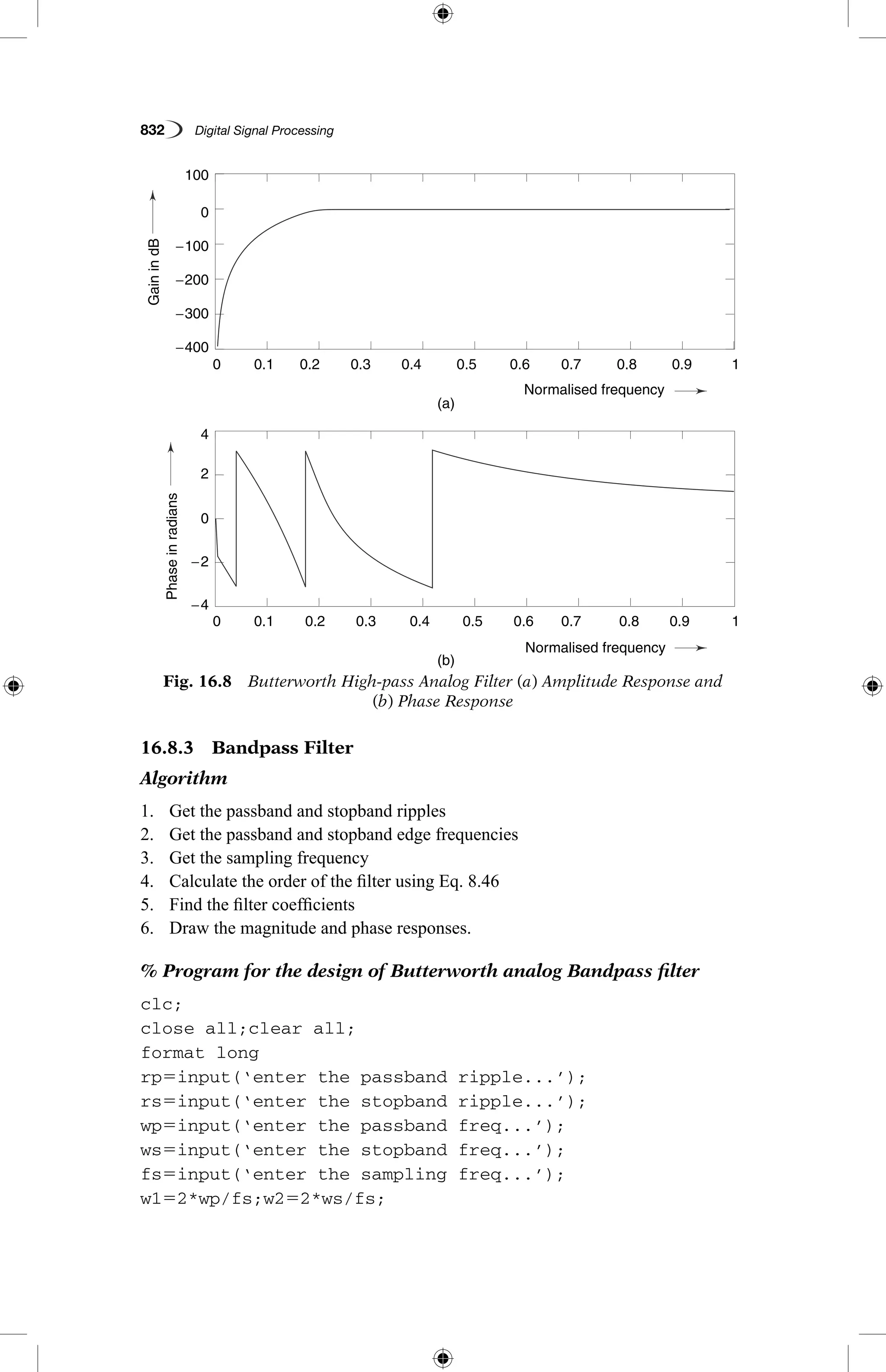
As an example,
enter the passband ripple 0.2
enter the stopband ripple 40
enter the passband freq 2000
enter the stopband freq 3500
enter the sampling freq 8000
The amplitude and phase responses of Butterworth high-pass analog filter are
shown in Fig. 16.8.](https://image.slidesharecdn.com/matlabprograms-150130053105-conversion-gate01/75/Matlab-programs-17-2048.jpg)
![MATLAB Programs 833
[n]5buttord(w1,w2,rp,rs);
wn5[w1 w2];
[b,a]5butter(n,wn,’bandpass’,’s’);
w50:.01:pi;
[h,om]5freqs(b,a,w);
m520*log10(abs(h));
an5angle(h);
subplot(2,1,1);plot(om/pi,m);
ylabel(‘Gain in dB --.’);xlabel(‘(a) Normalised
frequency --.’);
subplot(2,1,2);plot(om/pi,an);
xlabel(‘(b) Normalised frequency --.’);
ylabel(‘Phase in radians --.’);
As an example,
enter the passband ripple... 0.36
enter the stopband ripple... 36
enter the passband freq... 1500
enter the stopband freq... 2000
enter the sampling freq... 6000
The amplitude and phase responses of Butterworth bandpass analog filter are
shown in Fig. 16.9.
Fig. 16.9 Butterworth Bandpass Analog Filter (a) Amplitude Response and
(b) Phase Response
GainindB
Phaseinradians
(a)
(b)
0.1
0.1
−1000
−4
4
−2
2
0
−800
−600
−200
−400
0
200
0.2
0.2
0.3
0.3
0.4
0.4
Normalised frequency
Normalised frequency
0.5
0.5
0.6
0.6
0.7
0.7
0.8
0.8
0.9
0.9
1
1
0
0](https://image.slidesharecdn.com/matlabprograms-150130053105-conversion-gate01/75/Matlab-programs-19-2048.jpg)
![834 Digital Signal Processing
16.8.4 Bandstop Filter
Algorithm
1. Get the passband and stopband ripples
2. Get the passband and stopband edge frequencies
3. Get the sampling frequency
4. Calculate the order of the filter using Eq. 8.46
5. Find the filter coefficients
6. Draw the magnitude and phase responses.
% Program for the design of Butterworth analog Bandstop filter
clc;
close all;clear all;
format long
rp5input(‘enter the passband ripple...’);
rs5input(‘enter the stopband ripple...’);
wp5input(‘enter the passband freq...’);
ws5input(‘enter the stopband freq...’);
fs5input(‘enter the sampling freq...’);
w152*wp/fs;w252*ws/fs;
[n]5buttord(w1,w2,rp,rs,’s’);
wn5[w1 w2];
[b,a]5butter(n,wn,’stop’,’s’);
w50:.01:pi;
[h,om]5freqs(b,a,w);
m520*log10(abs(h));
an5angle(h);
subplot(2,1,1);plot(om/pi,m);
ylabel(‘Gain in dB --.’);xlabel(‘(a) Normalised
frequency --.’);
subplot(2,1,2);plot(om/pi,an);
xlabel(‘(b) Normalised frequency --.’);
ylabel(‘Phase in radians --.’);
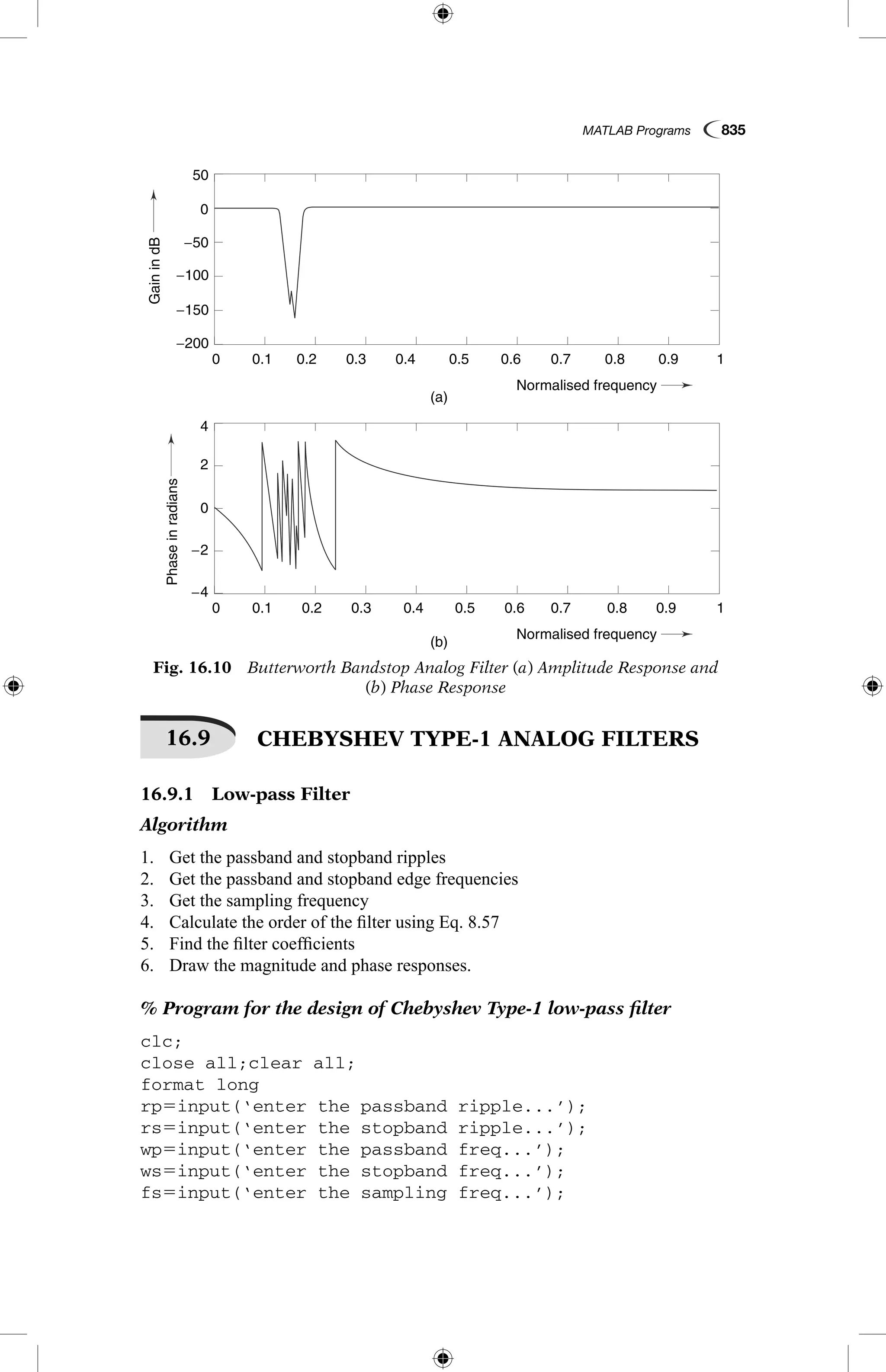
As an example,
enter the passband ripple... 0.28
enter the stopband ripple... 28
enter the passband freq... 1000
enter the stopband freq... 1400
enter the sampling freq... 5000
The amplitude and phase responses of Butterworth bandstop analog filter are
shown in Fig. 16.10.](https://image.slidesharecdn.com/matlabprograms-150130053105-conversion-gate01/75/Matlab-programs-20-2048.jpg)
![836 Digital Signal Processing
w152*wp/fs;w252*ws/fs;
[n,wn]5cheb1ord(w1,w2,rp,rs,’s’);
[b,a]5cheby1(n,rp,wn,’s’);
w50:.01:pi;
[h,om]5freqs(b,a,w);
m520*log10(abs(h));
an5angle(h);
subplot(2,1,1);plot(om/pi,m);
ylabel(‘Gain in dB --.’);xlabel(‘(a) Normalised
frequency --.’);
subplot(2,1,2);plot(om/pi,an);
xlabel(‘(b) Normalised frequency --.’);
ylabel(‘Phase in radians --.’);
As an example,
enter the passband ripple... 0.23
enter the stopband ripple... 47
enter the passband freq... 1300
enter the stopband freq... 1550
enter the sampling freq... 7800
The amplitude and phase responses of Chebyshev type - 1 low-pass analog filter
are shown in Fig. 16.11.
GainindBPhaseinradians
(a)
(b)
0.1
0.1
−4
4
−2
2
0
−80
−40
−20
−60
−100
0
0.2
0.2
0.3
0.3
0.4
0.4
Normalised frequency
Normalised frequency
0.5
0.5
0.6
0.6
0.7
0.7
0.8
0.8
0.9
0.9
1
1
0
0
Fig. 16.11 Chebyshev Type-I Low-pass Analog Filter (a) Amplitude Response
and (b) Phase Response](https://image.slidesharecdn.com/matlabprograms-150130053105-conversion-gate01/75/Matlab-programs-22-2048.jpg)
![MATLAB Programs 837
16.9.2 High-pass Filter
Algorithm
1. Get the passband and stopband ripples
2. Get the passband and stopband edge frequencies
3. Get the sampling frequency
4. Calculate the order of the filter using Eq. 8.57
5. Find the filter coefficients
6. Draw the magnitude and phase responses.
%Program for the design of Chebyshev Type-1 high-pass filter
clc;
close all;clear all;
format long
rp5input(‘enter the passband ripple...’);
rs5input(‘enter the stopband ripple...’);
wp5input(‘enter the passband freq...’);
ws5input(‘enter the stopband freq...’);
fs5input(‘enter the sampling freq...’);
w152*wp/fs;w252*ws/fs;
[n,wn]5cheb1ord(w1,w2,rp,rs,’s’);
[b,a]5cheby1(n,rp,wn,’high’,’s’);
w50:.01:pi;
[h,om]5freqs(b,a,w);
m520*log10(abs(h));
an5angle(h);
subplot(2,1,1);plot(om/pi,m);
Fig. 16.12 Chebyshev Type - 1 High-pass Analog Filter (a) Amplitude Response
and (b) Phase Response
GainindB
Phaseinradians
(a)
(b)
0.1
0.1
−4
4
−2
2
0
−100
−50
−150
−200
0
0.2
0.2
0.3
0.3
0.4
0.4
Normalised frequency
Normalised frequency
0.5
0.5
0.6
0.6
0.7
0.7
0.8
0.8
0.9
0.9
1
1
0
0
GainindB
Phaseinradians
(a)
(b)
0.1
0.1
−4
4
−2
2
0
−100
−50
−150
−200
0
0.2
0.2
0.3
0.3
0.4
0.4
Normalised frequency
Normalised frequency
0.5
0.5
0.6
0.6
0.7
0.7
0.8
0.8
0.9
0.9
1
1
0
0](https://image.slidesharecdn.com/matlabprograms-150130053105-conversion-gate01/75/Matlab-programs-23-2048.jpg)
![838 Digital Signal Processing
ylabel(‘Gain in dB --.’);xlabel(‘(a) Normalised
frequency --.’);
subplot(2,1,2);plot(om/pi,an);
xlabel(‘(b) Normalised frequency --.’);
ylabel(‘Phase in radians --.’);
As an example,
enter the passband ripple... 0.29
enter the stopband ripple... 29
enter the passband freq... 900
enter the stopband freq... 1300
enter the sampling freq... 7500
The amplitude and phase responses of Chebyshev type - 1 high-pass analog filter
are shown in Fig. 16.12.
16.9.3 Bandpass Filter
Algorithm
1. Get the passband and stopband ripples
2. Get the passband and stopband edge frequencies
3. Get the sampling frequency
4. Calculate the order of the filter using Eq. 8.57
5. Find the filter coefficients
6. Draw the magnitude and phase responses.
% Program for the design of Chebyshev Type-1 Bandpass filter
clc;
close all;clear all;
format long
rp5input(‘enter the passband ripple...’);
rs5input(‘enter the stopband ripple...’);
wp5input(‘enter the passband freq...’);
ws5input(‘enter the stopband freq...’);
fs5input(‘enter the sampling freq...’);
w152*wp/fs;w252*ws/fs;
[n]5cheb1ord(w1,w2,rp,rs,’s’);
wn5[w1 w2];
[b,a]5cheby1(n,rp,wn,’bandpass’,’s’);
w50:.01:pi;
[h,om]5freqs(b,a,w);
m520*log10(abs(h));
an5angle(h);
subplot(2,1,1);plot(om/pi,m);
ylabel(‘Gain in dB --.’);xlabel(‘(a) Normalised
frequency --.’);
subplot(2,1,2);plot(om/pi,an);
xlabel(‘(b) Normalised frequency --.’);
ylabel(‘Phase in radians --.’);
As an example,
enter the passband ripple... 0.3
enter the stopband ripple... 40
enter the passband freq... 1400](https://image.slidesharecdn.com/matlabprograms-150130053105-conversion-gate01/75/Matlab-programs-24-2048.jpg)
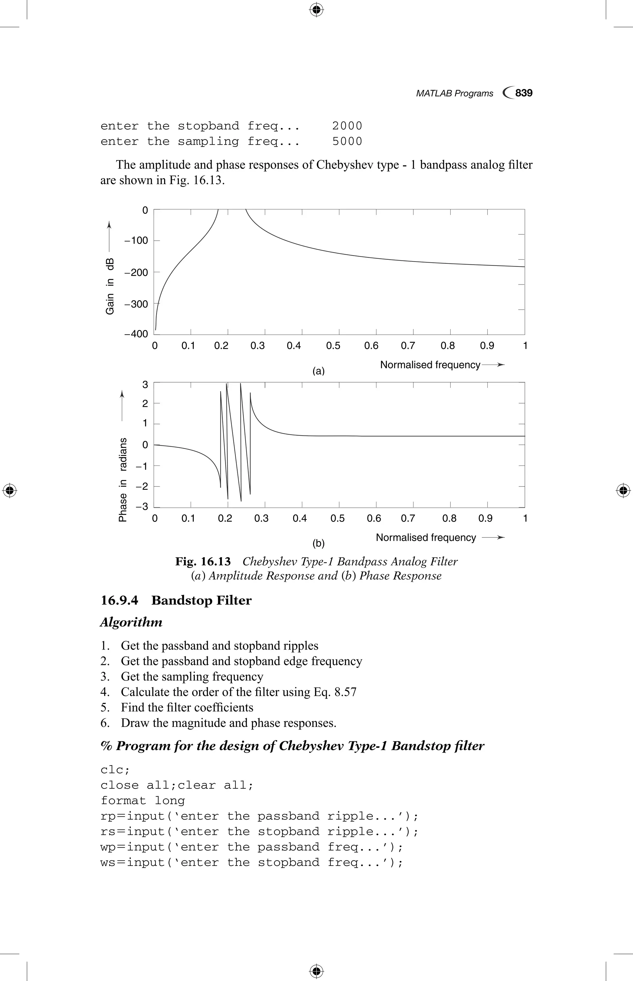
![840 Digital Signal Processing
fs5input(‘enter the sampling freq...’);
w152*wp/fs;w252*ws/fs;
[n]5cheb1ord(w1,w2,rp,rs,’s’);
wn5[w1 w2];
[b,a]5cheby1(n,rp,wn,’stop’,’s’);
w50:.01:pi;
[h,om]5freqs(b,a,w);
m520*log10(abs(h));
an5angle(h);
subplot(2,1,1);plot(om/pi,m);
ylabel(‘Gain in dB --.’);xlabel(‘(a) Normalised
frequency --.’);
subplot(2,1,2);plot(om/pi,an);
xlabel(‘(b) Normalised frequency --.’);
ylabel(‘Phase in radians --.’);
As an example,
enter the passband ripple... 0.15
enter the stopband ripple... 30
enter the passband freq... 2000
enter the stopband freq... 2400
enter the sampling freq... 7000
The amplitude and phase responses of Chebyshev type - 1 bandstop analog filter
are shown in Fig. 16.14.
Fig. 16.14 Chebyshev Type - 1 Bandstop Analog Filter
(a) Amplitude Response and (b) Phase Response
GainindB
Phaseinradians
(a)
(b)
0.1
0.1
−4
4
−2
2
0
−150
−50
−100
−200
−250
0
0.2
0.2
0.3
0.3
0.4
0.4
Normalised frequency
Normalised frequency
0.5
0.5
0.6
0.6
0.7
0.7
0.8
0.8
0.9
0.9
1
1
0
0
GainindB
Phaseinradians
(a)
(b)
0.1
0.1
−4
4
−2
2
0
−150
−50
−100
−200
−250
0
0.2
0.2
0.3
0.3
0.4
0.4
Normalised frequency
Normalised frequency
0.5
0.5
0.6
0.6
0.7
0.7
0.8
0.8
0.9
0.9
1
1
0
0](https://image.slidesharecdn.com/matlabprograms-150130053105-conversion-gate01/75/Matlab-programs-26-2048.jpg)
![MATLAB Programs 841
16.10 CHEBYSHEV TYPE-2 ANALOG FILTERS
16.10.1 Low-pass Filter
Algorithm
1. Get the passband and stopband ripples
2. Get the passband and stopband edge frequencies
3. Get the sampling frequency
4. Calculate the order of the filter using Eq. 8.67
5. Find the filter coefficients
6. Draw the magnitude and phase responses.
% Program for the design of Chebyshev Type-2 low pass analog filter
clc;
close all;clear all;
format long
rp5input(‘enter the passband ripple...’);
rs5input(‘enter the stopband ripple...’);
wp5input(‘enter the passband freq...’);
ws5input(‘enter the stopband freq...’);
fs5input(‘enter the sampling freq...’);
w152*wp/fs;w252*ws/fs;
[n,wn]5cheb2ord(w1,w2,rp,rs,’s’);
[b,a]5cheby2(n,rs,wn,’s’);
w50:.01:pi;
[h,om]5freqs(b,a,w);
m520*log10(abs(h));
an5angle(h);
subplot(2,1,1);plot(om/pi,m);
ylabel(‘Gain in dB --.’);xlabel(‘(a) Normalised
frequency --.’);
subplot(2,1,2);plot(om/pi,an);
xlabel(‘(b) Normalised frequency --.’);
ylabel(‘Phase in radians --.’);
As an example,
enter the passband ripple... 0.4
enter the stopband ripple... 50
enter the passband freq... 2000
enter the stopband freq... 2400
enter the sampling freq... 10000
The amplitude and phase responses of Chebyshev type - 2 low-pass analog filter
are shown in Fig. 16.15.](https://image.slidesharecdn.com/matlabprograms-150130053105-conversion-gate01/75/Matlab-programs-27-2048.jpg)
![842 Digital Signal Processing
Fig. 16.15 Chebyshev Type - 2 Low-pass Analog Filter (a) Amplitude Response
and (b) Phase Response
GainindB
Phaseinradians
(a)
(b)
0.1
0.1
−4
4
−2
2
0
−60
−20
−40
−80
−100
0
0.2
0.2
0.3
0.3
0.4
0.4
Normalised frequency
Normalised frequency
0.5
0.5
0.6
0.6
0.7
0.7
0.8
0.8
0.9
0.9
1
1
0
0
16.10.2 High-pass Filter
Algorithm
1. Get the passband and stopband ripples
2. Get the passband and stopband edge frequencies
3. Get the sampling frequency
4. Calculate the order of the filter using Eq. 8.67
5. Find the filter coefficients
6. Draw the magnitude and phase responses.
% Program for the design of Chebyshev Type-2 High pass analog filter
clc;
close all;clear all;
format long
rp5input(‘enter the passband ripple...’);
rs5input(‘enter the stopband ripple...’);
wp5input(‘enter the passband freq...’);
ws5input(‘enter the stopband freq...’);
fs5input(‘enter the sampling freq...’);
w152*wp/fs;w252*ws/fs;
[n,wn]5cheb2ord(w1,w2,rp,rs,’s’);
[b,a]5cheby2(n,rs,wn,’high’,’s’);
w50:.01:pi;](https://image.slidesharecdn.com/matlabprograms-150130053105-conversion-gate01/75/Matlab-programs-28-2048.jpg)
![MATLAB Programs 843
[h,om]5freqs(b,a,w);
m520*log10(abs(h));
an5angle(h);
subplot(2,1,1);plot(om/pi,m);
ylabel(‘Gain in dB --.’);xlabel(‘(a) Normalised frequency --.’);
subplot(2,1,2);plot(om/pi,an);
xlabel(‘(b) Normalised frequency --.’);
ylabel(‘Phase in radians --.’);
As an example,
enter the passband ripple... 0.34
enter the stopband ripple... 34
enter the passband freq... 1400
enter the stopband freq... 1600
enter the sampling freq... 10000
The amplitude and phase responses of Chebyshev type - 2 high-pass analog filter
are shown in Fig. 16.16.
GainindB
Phaseinradians
(a)
(b)
0.1
0.1
−4
4
−2
2
0
−60
−20
−40
−80
0
0.2
0.2
0.3
0.3
0.4
0.4
Normalised frequency
Normalised frequency
0.5
0.5
0.6
0.6
0.7
0.7
0.8
0.8
0.9
0.9
1
1
0
0
Fig. 16.16 Chebyshev Type - 2 High-pass Analog Filter
(a) Amplitude Response and (b) Phase Response
16.10.3 Bandpass Filter
Algorithm
1. Get the passband and stopband ripples
2. Get the passband and stopband edge frequencies](https://image.slidesharecdn.com/matlabprograms-150130053105-conversion-gate01/75/Matlab-programs-29-2048.jpg)
![844 Digital Signal Processing
3. Get the sampling frequency
4. Calculate the order of the filter using Eq. 8.67
5. Find the filter coefficients
6. Draw the magnitude and phase responses.
% Program for the design of Chebyshev Type-2 Bandpass analog filter
clc;
close all;clear all;
format long
rp5input(‘enter the passband ripple...’);
rs5input(‘enter the stopband ripple...’);
wp5input(‘enter the passband freq...’);
ws5input(‘enter the stopband freq...’);
fs5input(‘enter the sampling freq...’);
w152*wp/fs;w252*ws/fs;
[n]5cheb2ord(w1,w2,rp,rs,’s’);
wn5[w1 w2];
[b,a]5cheby2(n,rs,wn,’bandpass’,’s’);
w50:.01:pi;
[h,om]5freqs(b,a,w);
m520*log10(abs(h));
an5angle(h);
subplot(2,1,1);plot(om/pi,m);
ylabel(‘Gain in dB --.’);xlabel(‘(a) Normalised
frequency --.’);
subplot(2,1,2);plot(om/pi,an);
xlabel(‘(b) Normalised frequency --.’);
ylabel(‘Phase in radians --.’);
As an example,
enter the passband ripple... 0.37
enter the stopband ripple... 37
enter the passband freq... 3000
enter the stopband freq... 4000
enter the sampling freq... 9000
The amplitude and phase responses of Chebyshev type - 2 bandpass analog filter
are shown in Fig. 16.17.
Fig. 16.17 (Contd.)
GainindB
aseinradians
(a)
0.1
4
−2
2
0
−80
−60
−20
0
−40
−100
20
0.2 0.3 0.4
Normalised frequency
0.5 0.6 0.7 0.8 0.9 10](https://image.slidesharecdn.com/matlabprograms-150130053105-conversion-gate01/75/Matlab-programs-30-2048.jpg)
![MATLAB Programs 845
16.10.4 Bandstop Filter
Algorithm
1. Get the passband and stopband ripples
2. Get the passband and stopband edge frequencies
3. Get the sampling frequency
4. Calculate the order of the filter using Eq. 8.67
5. Find the filter coefficients
6. Draw the magnitude and phase responses.
% Program for the design of Chebyshev Type-2 Bandstop analog filter
clc;
close all;clear all;
format long
rp5input(‘enter the passband ripple...’);
rs5input(‘enter the stopband ripple...’);
wp5input(‘enter the passband freq...’);
ws5input(‘enter the stopband freq...’);
fs5input(‘enter the sampling freq...’);
w152*wp/fs;w252*ws/fs;
[n]5cheb2ord(w1,w2,rp,rs,’s’);
wn5[w1 w2];
[b,a]5cheby2(n,rs,wn,’stop’,’s’);
w50:.01:pi;
[h,om]5freqs(b,a,w);
m520*log10(abs(h));
an5angle(h);
subplot(2,1,1);plot(om/pi,m);
ylabel(‘Gain in dB --.’);xlabel(‘(a) Normalised
frequency --.’);
subplot(2,1,2);plot(om/pi,an);
xlabel(‘(b) Normalised frequency --.’);
ylabel(‘Phase in radians --.’);
Fig. 16.17 Chebyshev Type - 2 Bandstop Analog Filter (a) Amplitude Response
and (b) Phase Response
Gainind
Phaseinradians
(a)
(b)
0.1
0.1
−4
4
−2
2
0
−80
−60
−40
−100
0.2
0.2
0.3
0.3
0.4
0.4
Normalised frequency
Normalised frequency
0.5
0.5
0.6
0.6
0.7
0.7
0.8
0.8
0.9
0.9
1
1
0
0](https://image.slidesharecdn.com/matlabprograms-150130053105-conversion-gate01/75/Matlab-programs-31-2048.jpg)
![MATLAB Programs 847
% Program for the design of Butterworth low pass digital filter
clc;
close all;clear all;
format long
rp5input(‘enter the passband ripple’);
rs5input(‘enter the stopband ripple’);
wp5input(‘enter the passband freq’);
ws5input(‘enter the stopband freq’);
fs5input(‘enter the sampling freq’);
w152*wp/fs;w252*ws/fs;
[n,wn]5buttord(w1,w2,rp,rs);
[b,a]5butter(n,wn);
w50:.01:pi;
[h,om]5freqz(b,a,w);
m520*log10(abs(h));
an5angle(h);
subplot(2,1,1);plot(om/pi,m);
ylabel(‘Gain in dB --.’);xlabel(‘(a) Normalised
frequency --.’);
subplot(2,1,2);plot(om/pi,an);
xlabel(‘(b) Normalised frequency --.’);
ylabel(‘Phase in radians --.’);
As an example,
enter the passband ripple 0.5
enter the stopband ripple 50
enter the passband freq 1200
enter the stopband freq 2400
enter the sampling freq 10000
The amplitude and phase responses of Butterworth low-pass digital filter are
shown in Fig. 16.19.
GainindB
Phaseinradians
(a)
0.1
0.1
−4
4
−2
2
0
−300
−200
0
−100
−400
100
0.2
0.2
0.3
0.3
0.4
0.4
Normalised frequency
0.5
0.5
0.6
0.6
0.7
0.7
0.8
0.8
0.9
0.9
1
1
0
0
Fig. 16.19 (Contd.)](https://image.slidesharecdn.com/matlabprograms-150130053105-conversion-gate01/75/Matlab-programs-33-2048.jpg)
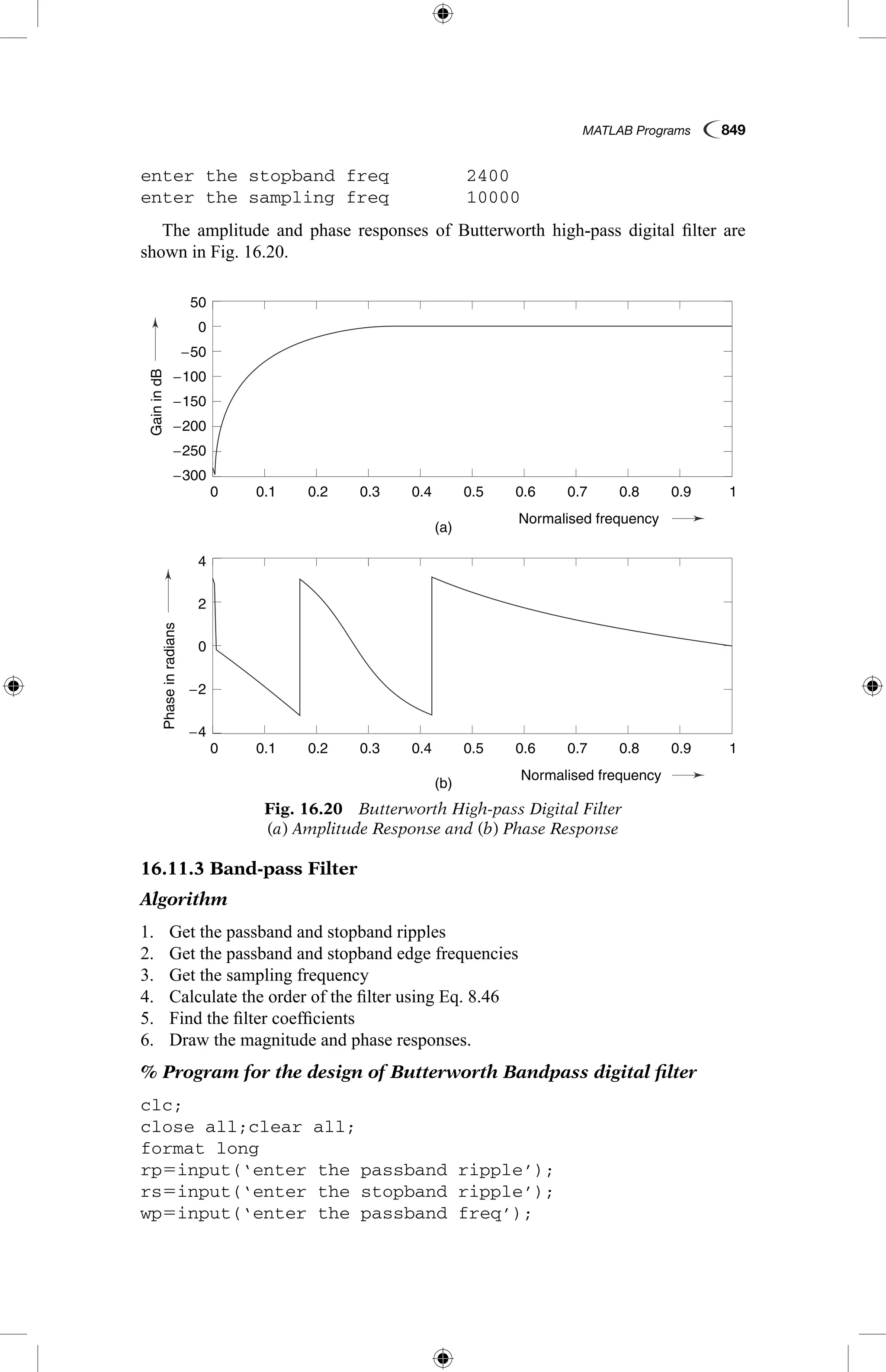
![848 Digital Signal Processing
16.11.2 High-pass Filter
Algorithm
1. Get the passband and stopband ripples
2. Get the passband and stopband edge frequencies
3. Get the sampling frequency
4. Calculate the order of the filter using Eq. 8.46
5. Find the filter coefficients
6. Draw the magnitude and phase responses.
% Program for the design of Butterworth highpass digital filter
clc;
close all;clear all;
format long
rp5input(‘enter the passband ripple’);
rs5input(‘enter the stopband ripple’);
wp5input(‘enter the passband freq’);
ws5input(‘enter the stopband freq’);
fs5input(‘enter the sampling freq’);
w152*wp/fs;w252*ws/fs;
[n,wn]5buttord(w1,w2,rp,rs);
[b,a]5butter(n,wn,’high’);
w50:.01:pi;
[h,om]5freqz(b,a,w);
m520*log10(abs(h));
an5angle(h);
subplot(2,1,1);plot(om/pi,m);
ylabel(‘Gain in dB --.’);xlabel(‘(a) Normalised
frequency --.’);
subplot(2,1,2);plot(om/pi,an);
xlabel(‘(b) Normalised frequency --.’);
ylabel(‘Phase in radians --.’);
As an example,
enter the passband ripple 0.5
enter the stopband ripple 50
enter the passband freq 1200
Fig. 16.19 Butterworth Low-pass Digital Filter (a) Amplitude Response and
(b) Phase Response
Gain
Phaseinradians
(a)
(b)
0.1
0.1
−4
4
−2
2
0
−300
−200
−400
0.2
0.2
0.3
0.3
0.4
0.4
Normalised frequency
Normalised frequency
0.5
0.5
0.6
0.6
0.7
0.7
0.8
0.8
0.9
0.9
1
1
0
0](https://image.slidesharecdn.com/matlabprograms-150130053105-conversion-gate01/75/Matlab-programs-34-2048.jpg)
![850 Digital Signal Processing
ws5input(‘enter the stopband freq’);
fs5input(‘enter the sampling freq’);
w152*wp/fs;w252*ws/fs;
[n]5buttord(w1,w2,rp,rs);
wn5[w1 w2];
[b,a]5butter(n,wn,’bandpass’);
w50:.01:pi;
[h,om]5freqz(b,a,w);
m520*log10(abs(h));
an5angle(h);
subplot(2,1,1);plot(om/pi,m);
ylabel(‘Gain in dB --.’);xlabel(‘(a) Normalised
frequency --.’);
subplot(2,1,2);plot(om/pi,an);
xlabel(‘(b) Normalised frequency --.’);
ylabel(‘Phase in radians --.’);
As an example,
enter the passband ripple 0.3
enter the stopband ripple 40
enter the passband freq 1500
enter the stopband freq 2000
enter the sampling freq 9000
The amplitude and phase responses of Butterworth band-pass digital filter are
shown in Fig. 16.21.
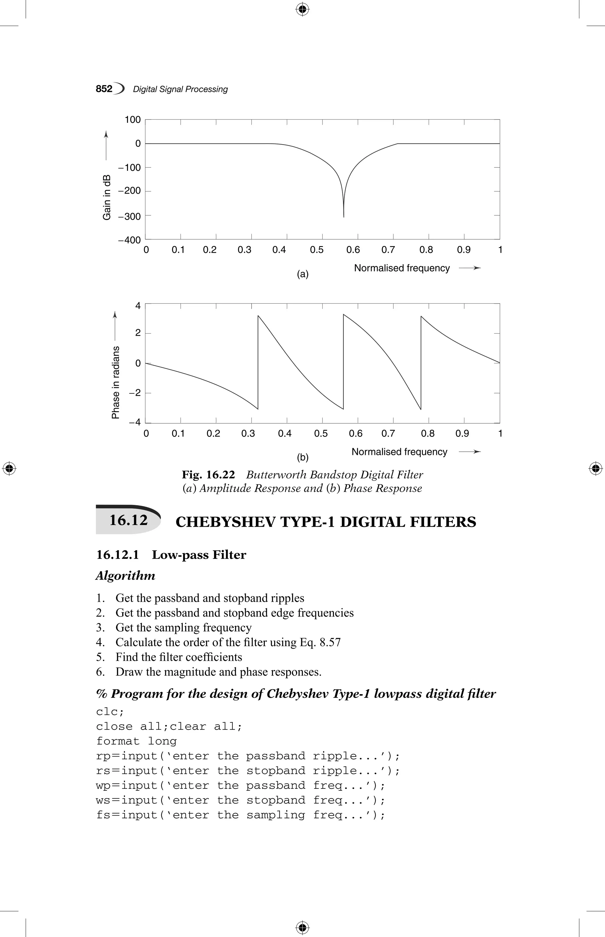
Fig. 16.21 Butterworth Bandstop Digital Filter (a) Amplitude Response and
(b) Phase Response
GainindB
(a)
(b)
Phaseinradians
0.1
0.1
0
− 200
− 100
− 400
− 500
− 600
− 700
4
2
0
− 2
− 4
− 300
0.2
0.2
0.3
0.3
0.4
0.4
Normalised frequency
Normalised frequency
0.5
0.5
0.6
0.6
0.7
0.7
0.8
0.8
0.9
0.9
1
1
0
0](https://image.slidesharecdn.com/matlabprograms-150130053105-conversion-gate01/75/Matlab-programs-36-2048.jpg)
![MATLAB Programs 851
16.11.4 Bandstop Filter
Algorithm
1. Get the passband and stopband ripples
2. Get the passband and stopband edge frequencies
3. Get the sampling frequency
4. Calculate the order of the filter using Eq. 8.46
5. Find the filter coefficients
6. Draw the magnitude and phase responses.
% Program for the design of Butterworth Band stop digital filter
clc;
close all;clear all;
format long
rp5input(‘enter the passband ripple’);
rs5input(‘enter the stopband ripple’);
wp5input(‘enter the passband freq’);
ws5input(‘enter the stopband freq’);
fs5input(‘enter the sampling freq’);
w152*wp/fs;w252*ws/fs;
[n]5buttord(w1,w2,rp,rs);
wn5[w1 w2];
[b,a]5butter(n,wn,’stop’);
w50:.01:pi;
[h,om]5freqz(b,a,w);
m520*log10(abs(h));
an5angle(h);
subplot(2,1,1);plot(om/pi,m);
ylabel(‘Gain in dB --.’);xlabel(‘(a) Normalised
frequency --.’);
subplot(2,1,2);plot(om/pi,an);
xlabel(‘(b) Normalised frequency --.’);
ylabel(‘Phase in radians --.’);
As an example,
enter the passband ripple 0.4
enter the stopband ripple 46
enter the passband freq 1100
enter the stopband freq 2200
enter the sampling freq 6000
The amplitude and phase responses of the Butterworth bandstop digital filter are
shown in Fig. 16.22.](https://image.slidesharecdn.com/matlabprograms-150130053105-conversion-gate01/75/Matlab-programs-37-2048.jpg)
![MATLAB Programs 853
w152*wp/fs;w252*ws/fs;
[n,wn]5cheb1ord(w1,w2,rp,rs);
[b,a]5cheby1(n,rp,wn);
w50:.01:pi;
[h,om]5freqz(b,a,w);
m520*log10(abs(h));
an5angle(h);
subplot(2,1,1);plot(om/pi,m);
ylabel(‘Gain in dB --.’);xlabel(‘(a) Normalised
frequency --.’);
subplot(2,1,2);plot(om/pi,an);
xlabel(‘(b) Normalised frequency --.’);
ylabel(‘Phase in radians --.’);
As an example,
enter the passband ripple... 0.2
enter the stopband ripple... 45
enter the passband freq... 1300
enter the stopband freq... 1500
enter the sampling freq... 10000
The amplitude and phase responses of Chebyshev type - 1 low-pass digital filter
are shown in Fig. 16.23.
Fig. 16.23 Chebyshev Type - 1 Low-pass Digital Filter (a) Amplitude Response
and (b) Phase Response
GainindB
Phaseinradians
(a)
(b)
0.1
0.1
−4
4
−2
2
0
0
−200
−100
−500
−400
−300
0.2
0.2
0.3
0.3
0.4
0.4
Normalised frequency
Normalised frequency
0.5
0.5
0.6
0.6
0.7
0.7
0.8
0.8
0.9
0.9
1
1
0
0](https://image.slidesharecdn.com/matlabprograms-150130053105-conversion-gate01/75/Matlab-programs-39-2048.jpg)
![854 Digital Signal Processing
16.12.2 High-pass Filter
Algorithm
1. Get the passband and stopband ripples
2. Get the passband and stopband edge frequencies
3. Get the sampling frequency
4. Calculate the order of the filter using Eq. 8.57
5. Find the filter coefficients
6. Draw the magnitude and phase responses.
% Program for the design of Chebyshev Type-1 highpass digital
filter
clc;
close all;clear all;
format long
rp5input(‘enter the passband ripple...’);
rs5input(‘enter the stopband ripple...’);
wp5input(‘enter the passband freq...’);
ws5input(‘enter the stopband freq...’);
fs5input(‘enter the sampling freq...’);
w152*wp/fs;w252*ws/fs;
[n,wn]5cheb1ord(w1,w2,rp,rs);
[b,a]5cheby1(n,rp,wn,’high’);
w50:.01/pi:pi;
[h,om]5freqz(b,a,w);
m520*log10(abs(h));
an5angle(h);
subplot(2,1,1);plot(om/pi,m);
ylabel(‘Gain in dB --.’);xlabel(‘(a) Normalised frequency
--.’);
subplot(2,1,2);plot(om/pi,an);
xlabel(‘(b) Normalised frequency --.’);
ylabel(‘Phase in radians --.’);
As an example,
enter the passband ripple... 0.3
enter the stopband ripple... 60
enter the passband freq... 1500
enter the stopband freq... 2000
enter the sampling freq... 9000
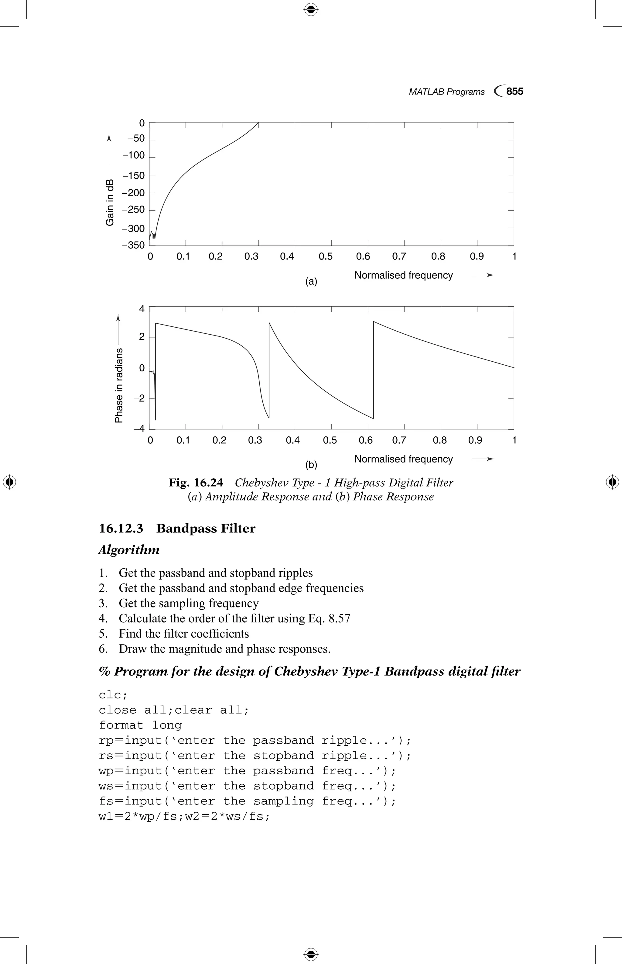
The amplitude and phase responses of Chebyshev type - 1 high-pass digital filter
are shown in Fig. 16.24.](https://image.slidesharecdn.com/matlabprograms-150130053105-conversion-gate01/75/Matlab-programs-40-2048.jpg)
![856 Digital Signal Processing
[n]5cheb1ord(w1,w2,rp,rs);
wn5[w1 w2];
[b,a]5cheby1(n,rp,wn,’bandpass’);
w50:.01:pi;
[h,om]5freqz(b,a,w);
m520*log10(abs(h));
an5angle(h);
subplot(2,1,1);plot(om/pi,m);
ylabel(‘Gain in dB --.’);xlabel(‘(a) Normalised
frequency --.’);
subplot(2,1,2);plot(om/pi,an);
xlabel(‘(b) Normalised frequency --.’);
ylabel(‘Phase in radians --.’);
As an example,
enter the passband ripple... 0.4
enter the stopband ripple... 35
enter the passband freq... 2000
enter the stopband freq... 2500
enter the sampling freq... 10000
The amplitude and phase responses of Chebyshev type - 1 bandpass digital filter
are shown in Fig. 16.25.
GainindB
Phaseinradians
(a)
(b)
0.1
0.1
−4
4
−2
2
0
0
−300
−200
−100
−500
−400
0.2
0.2
0.3
0.3
0.4
0.4
Normalised frequency
Normalised frequency
0.5
0.5
0.6
0.6
0.7
0.7
0.8
0.8
0.9
0.9
1
1
0
0
Fig. 16.25 Chebyshev Type - 1 Bandpass Digital Filter (a) Amplitude
Response and (b) Phase Response](https://image.slidesharecdn.com/matlabprograms-150130053105-conversion-gate01/75/Matlab-programs-42-2048.jpg)
![MATLAB Programs 857
16.12.4 Bandstop Filter
Algorithm
1. Get the passband and stopband ripples
2. Get the passband and stopband edge frequencies
3. Get the sampling frequency
4. Calculate the order of the filter using Eq. 8.57
5. Find the filter coefficients
6. Draw the magnitude and phase responses.
% Program for the design of Chebyshev Type-1 Bandstop digital filter
clc;
close all;clear all;
format long
rp5input(‘enter the passband ripple...’);
rs5input(‘enter the stopband ripple...’);
wp5input(‘enter the passband freq...’);
ws5input(‘enter the stopband freq...’);
fs5input(‘enter the sampling freq...’);
w152*wp/fs;w252*ws/fs;
[n]5cheb1ord(w1,w2,rp,rs);
wn5[w1 w2];
[b,a]5cheby1(n,rp,wn,’stop’);
w50:.1/pi:pi;
[h,om]5freqz(b,a,w);
m520*log10(abs(h));
an5angle(h);
subplot(2,1,1);plot(om/pi,m);
ylabel(‘Gain in dB --.’);xlabel(‘(a) Normalised
frequency --.’);
subplot(2,1,2);plot(om/pi,an);
xlabel(‘(b) Normalised frequency --.’);
ylabel(‘Phase in radians --.’);
As an example,
enter the passband ripple... 0.25
enter the stopband ripple... 40
enter the passband freq... 2500
enter the stopband freq... 2750
enter the sampling freq... 7000
The amplitude and phase responses of Chebyshev type - 1 bandstop digital filter
are shown in Fig. 16.26.](https://image.slidesharecdn.com/matlabprograms-150130053105-conversion-gate01/75/Matlab-programs-43-2048.jpg)
![858 Digital Signal Processing
Fig. 16.26 Chebyshev Type - 1 Bandstop Digital Filter
(a) Amplitude Response and (b) Phase Response
GainindB
Phaseinradians
(a)
(b)
0.1
0.1
−3
−2
−1
1
2
3
4
0
0
− 200
− 150
− 100
−50
0.2
0.2
0.3
0.3
0.4
0.4
Normalised frequency
Normalised frequency
0.5
0.5
0.6
0.6
0.7
0.7
0.8
0.8
0.9
0.9
1
1
0
0
GainindB
Phaseinradians
(a)
(b)
0.1
0.1
−3
−2
−1
1
2
3
4
0
0
− 200
− 150
− 100
−50
0.2
0.2
0.3
0.3
0.4
0.4
Normalised frequency
Normalised frequency
0.5
0.5
0.6
0.6
0.7
0.7
0.8
0.8
0.9
0.9
1
1
0
0
16.13 CHEBYSHEV TYPE-2 DIGITAL FILTERS
16.13.1 Low-pass Filter
Algorithm
1. Get the passband and stopband ripples
2. Get the passband and stopband edge frequencies
3. Get the sampling frequency
4. Calculate the order of the filter using Eq. 8.67
5. Find the filter coefficients
6. Draw the magnitude and phase responses.
% Program for the design of Chebyshev Type-2 lowpass digital filter
clc;
close all;clear all;
format long
rp5input(‘enter the passband ripple...’);
rs5input(‘enter the stopband ripple...’);
wp5input(‘enter the passband freq...’);
ws5input(‘enter the stopband freq...’);
fs5input(‘enter the sampling freq...’);
w152*wp/fs;w252*ws/fs;
[n,wn]5cheb2ord(w1,w2,rp,rs);
[b,a]5cheby2(n,rs,wn);](https://image.slidesharecdn.com/matlabprograms-150130053105-conversion-gate01/75/Matlab-programs-44-2048.jpg)
![MATLAB Programs 859
w50:.01:pi;
[h,om]5freqz(b,a,w);
m520*log10(abs(h));
an5angle(h);
subplot(2,1,1);plot(om/pi,m);
ylabel(‘Gain in dB --.’);xlabel(‘(a) Normalised
frequency --.’);
subplot(2,1,2);plot(om/pi,an);
xlabel(‘(b) Normalised frequency --.’);
ylabel(‘Phase in radians --.’);
As an example,
enter the passband ripple... 0.35
enter the stopband ripple... 35
enter the passband freq... 1500
enter the stopband freq... 2000
enter the sampling freq... 8000
The amplitude and phase responses of Chebyshev type - 2 low-pass digital filter
are shown in Fig. 16.27.
Fig. 16.27 Chebyshev Type - 2 Low-pass Digital Filter (a) Amplitude Response
and (b) Phase Response
GainindB
Phaseinradians
(a)
(b)
0.1
0.1
−4
−2
2
4
0
−100
−80
−60
−40
−20
0
20
0.2
0.2
0.3
0.3
0.4
0.4
Normalised frequency
Normalised frequency
0.5
0.5
0.6
0.6
0.7
0.7
0.8
0.8
0.9
0.9
1
1
0
0
GainindB
Phaseinradians
(a)
(b)
0.1
0.1
−4
−2
2
4
0
−100
−80
−60
−40
−20
0
20
0.2
0.2
0.3
0.3
0.4
0.4
Normalised frequency
Normalised frequency
0.5
0.5
0.6
0.6
0.7
0.7
0.8
0.8
0.9
0.9
1
1
0
0
16.13.2 High-pass Filter
Algorithm
1. Get the passband and stopband ripples
2. Get the passband and stopband edge frequencies](https://image.slidesharecdn.com/matlabprograms-150130053105-conversion-gate01/75/Matlab-programs-45-2048.jpg)
![860 Digital Signal Processing
3. Get the sampling frequency
4. Calculate the order of the filter using Eq. 8.67
5. Find the filter coefficients
6. Draw the magnitude and phase responses.
% Program for the design of Chebyshev Type-2 high pass digital filter
clc;
close all;clear all;
format long
rp5input(‘enter the passband ripple...’);
rs5input(‘enter the stopband ripple...’);
wp5input(‘enter the passband freq...’);
ws5input(‘enter the stopband freq...’);
fs5input(‘enter the sampling freq...’);
w152*wp/fs;w252*ws/fs;
[n,wn]5cheb2ord(w1,w2,rp,rs);
[b,a]5cheby2(n,rs,wn,’high’);
w50:.01/pi:pi;
[h,om]5freqz(b,a,w);
m520*log10(abs(h));
an5angle(h);
subplot(2,1,1);plot(om/pi,m);
ylabel(‘Gain in dB --.’);xlabel(‘(a) Normalised
frequency --.’);
subplot(2,1,2);plot(om/pi,an);
xlabel(‘(b) Normalised frequency --.’);
ylabel(‘Phase in radians --.’);
As an example,
enter the passband ripple... 0.25
enter the stopband ripple... 40
enter the passband freq... 1400
enter the stopband freq... 1800
enter the sampling freq... 7000
The amplitude and phase responses of Chebyshev type - 2 high-pass digital filter
are shown in Fig. 16.28.
GainindB
aseinradians
(a)
0.1
−2
2
4
0
−120
−100
−80
−60
−40
−20
0
0.2 0.3 0.4
Normalised frequency
0.5 0.6 0.7 0.8 0.9 10
Fig. 16.28 (Contd.)](https://image.slidesharecdn.com/matlabprograms-150130053105-conversion-gate01/75/Matlab-programs-46-2048.jpg)
![MATLAB Programs 861
16.13.3 Bandpass Filter
Algorithm
1. Get the passband and stopband ripples
2. Get the passband and stopband edge frequency
3. Get the sampling frequency
4. Calculate the order of the filter using Eq. 8.67
5. Find the filter coefficients
6. Draw the magnitude and phase responses.
% Program for the design of Chebyshev Type-2 Bandpass digital filter
clc;
close all;clear all;
format long
rp5input(‘enter the passband ripple...’);
rs5input(‘enter the stopband ripple...’);
wp5input(‘enter the passband freq...’);
ws5input(‘enter the stopband freq...’);
fs5input(‘enter the sampling freq...’);
w152*wp/fs;w252*ws/fs;
[n]5cheb2ord(w1,w2,rp,rs);
wn5[w1 w2];
[b,a]5cheby2(n,rs,wn,’bandpass’);
w50:.01/pi:pi;
[h,om]5freqz(b,a,w);
m520*log10(abs(h));
an5angle(h);
subplot(2,1,1);plot(om/pi,m);
ylabel(‘Gain in dB --.’);xlabel(‘(a) Normalised
frequency --.’);
subplot(2,1,2);plot(om/pi,an);
xlabel(‘(b) Normalised frequency --.’);
ylabel(‘Phase in radians --.’);
Gainin
Phaseinradians
(a)
(b)
0.1
0.1
−4
−2
2
4
0
−120
−100
−80
0.2
0.2
0.3
0.3
0.4
0.4
Normalised frequency
Normalised frequency
0.5
0.5
0.6
0.6
0.7
0.7
0.8
0.8
0.9
0.9
1
1
0
0
Fig. 16.28 Chebyshev Type - 2 High-pass Digital Filter (a) Amplitude Response
and (b) Phase Response](https://image.slidesharecdn.com/matlabprograms-150130053105-conversion-gate01/75/Matlab-programs-47-2048.jpg)
![MATLAB Programs 863
% Program for the design of Chebyshev Type-2 Bandstop digital filter
clc;
close all;clear all;
format long
rp5input(‘enter the passband ripple...’);
rs5input(‘enter the stopband ripple...’);
wp5input(‘enter the passband freq...’);
ws5input(‘enter the stopband freq...’);
fs5input(‘enter the sampling freq...’);
w152*wp/fs;w252*ws/fs;
[n]5cheb2ord(w1,w2,rp,rs);
wn5[w1 w2];
[b,a]5cheby2(n,rs,wn,’stop’);
w50:.1/pi:pi;
[h,om]5freqz(b,a,w);
m520*log10(abs(h));
an5angle(h);
subplot(2,1,1);plot(om/pi,m);
ylabel(‘Gain in dB --.’);xlabel(‘(a) Normalised
frequency --.’);
subplot(2,1,2);plot(om/pi,an);
xlabel(‘(b) Normalised frequency --.’);
ylabel(‘Phase in radians --.’);
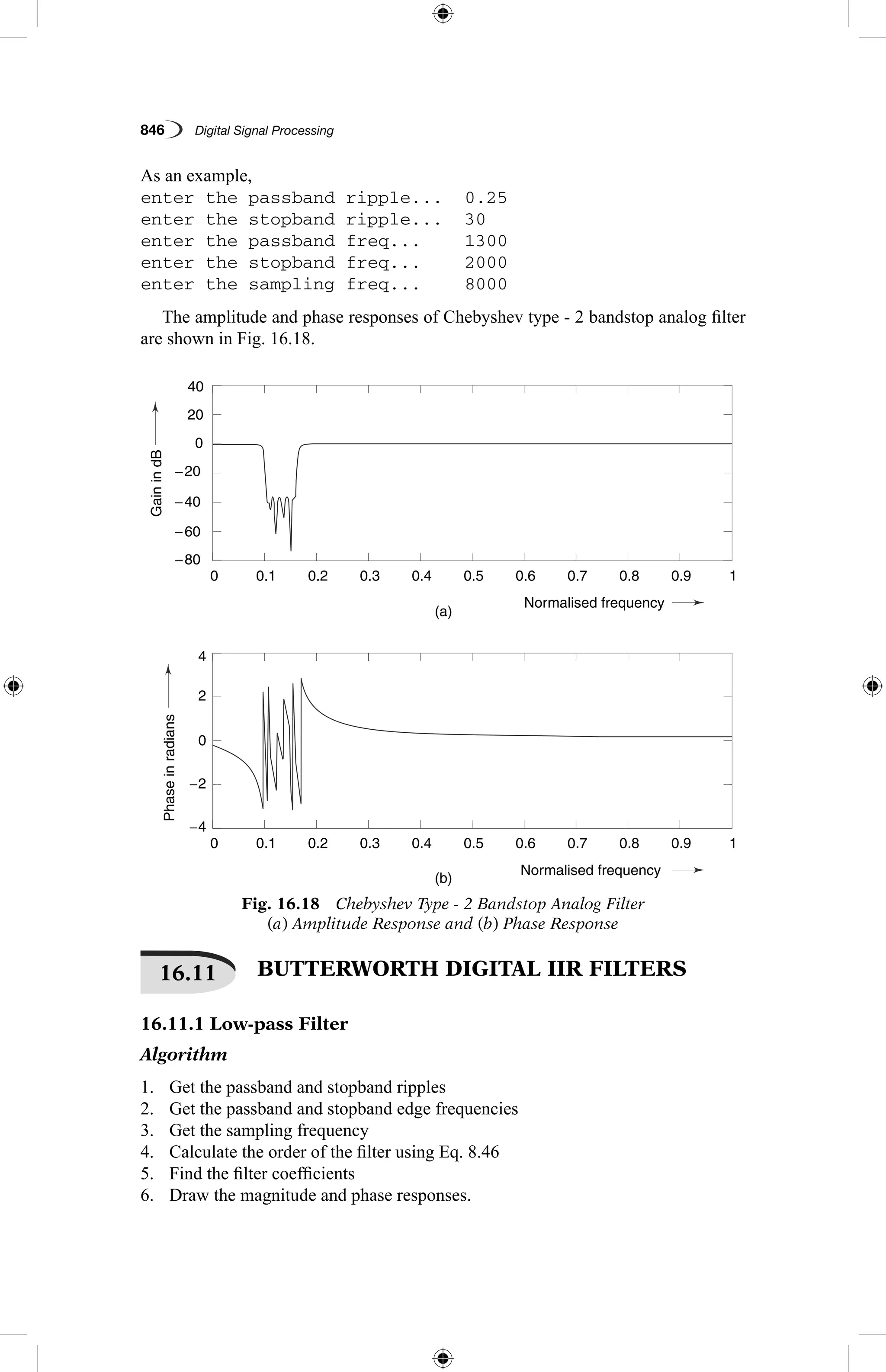
As an example,
enter the passband ripple... 0.3
enter the stopband ripple... 46
enter the passband freq... 1400
enter the stopband freq... 2000
enter the sampling freq... 8000
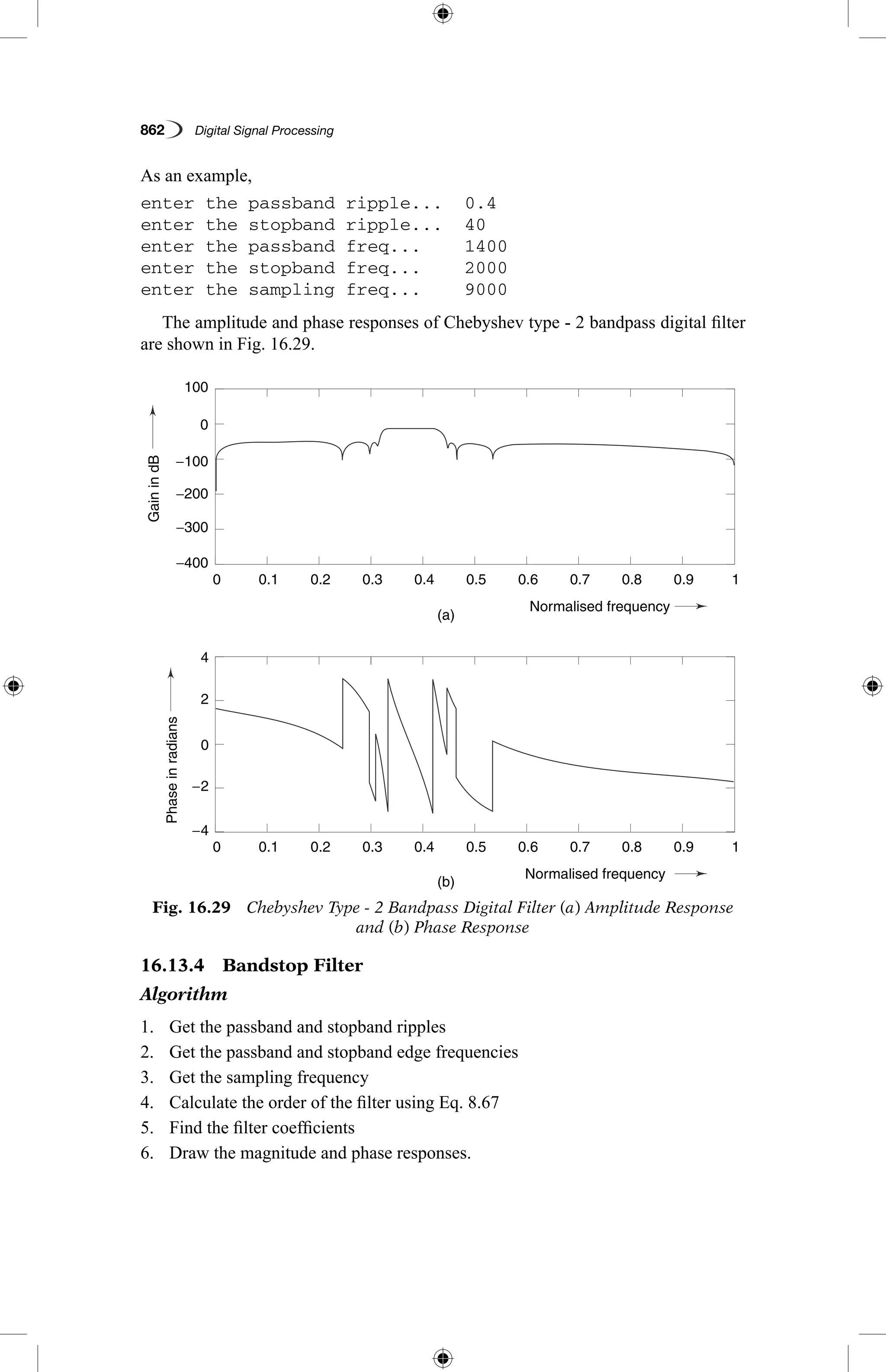
The amplitude and phase responses of Chebyshev type - 2 bandstop digital filter
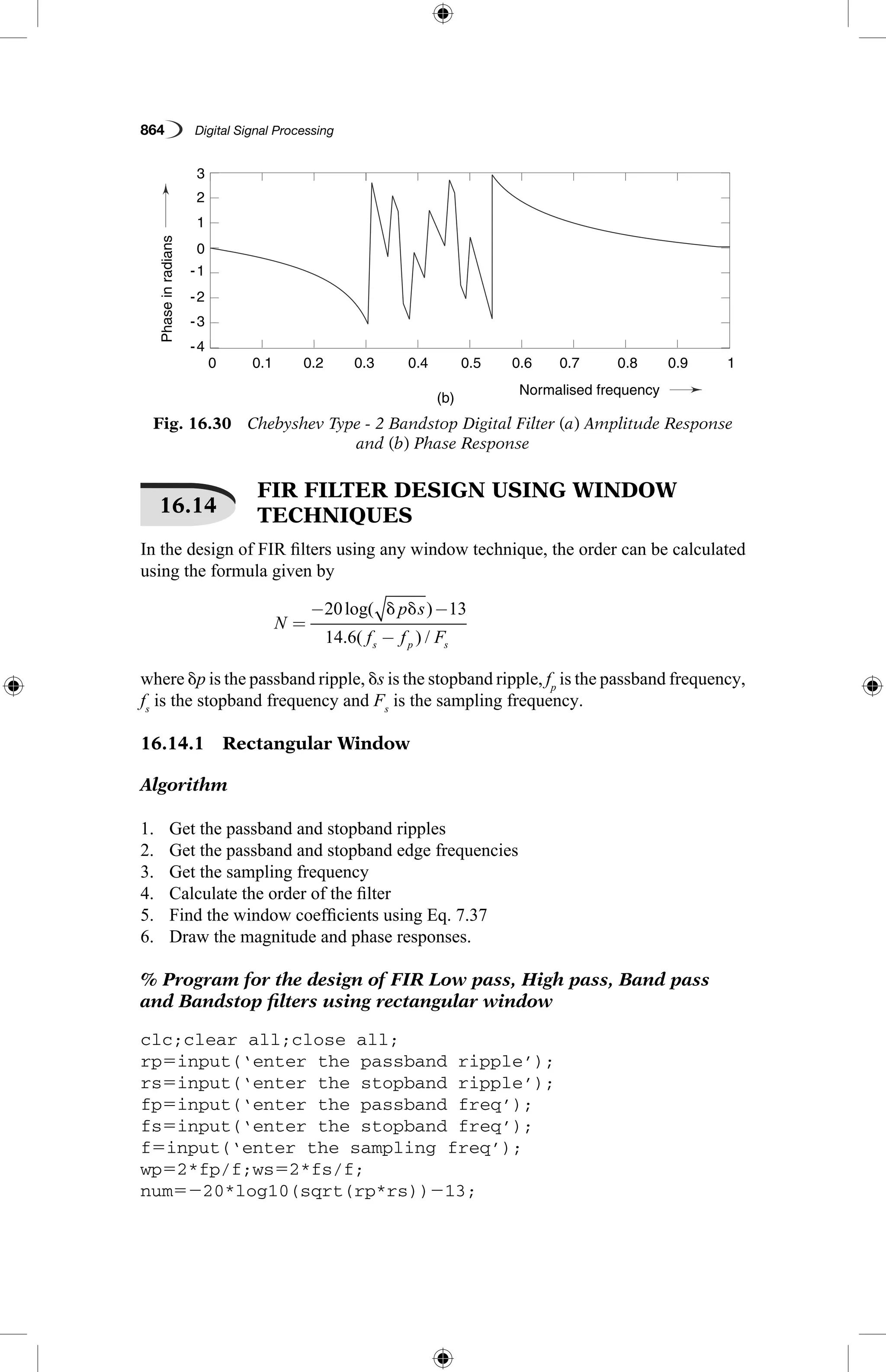
are shown in Fig. 16.30.
GainindB
Phaseinradians
(a)
0.1
-4
-2
-1
-3
3
0
1
2
−80
−60
−40
−20
0
20
0.2 0.3 0.4
Normalised frequency
0.5 0.6 0.7 0.8 0.9 10
Fig. 16.30 (Contd.)](https://image.slidesharecdn.com/matlabprograms-150130053105-conversion-gate01/75/Matlab-programs-49-2048.jpg)
![MATLAB Programs 865
dem514.6*(fs2fp)/f;
n5ceil(num/dem);
n15n11;
if (rem(n,2)˜50)
n15n;
n5n21;
end
y5boxcar(n1);
% low-pass filter
b5fir1(n,wp,y);
[h,o]5freqz(b,1,256);
m520*log10(abs(h));
subplot(2,2,1);plot(o/pi,m);ylabel(‘Gain in dB --.’);
xlabel(‘(a) Normalised frequency --.’);
% high-pass filter
b5fir1(n,wp,’high’,y);
[h,o]5freqz(b,1,256);
m520*log10(abs(h));
subplot(2,2,2);plot(o/pi,m);ylabel(‘Gain in dB --.’);
xlabel(‘(b) Normalised frequency --.’);
% band pass filter
wn5[wp ws];
b5fir1(n,wn,y);
[h,o]5freqz(b,1,256);
m520*log10(abs(h));
subplot(2,2,3);plot(o/pi,m);ylabel(‘Gain in dB --’);
xlabel(‘(c) Normalised frequency --’);
% band stop filter
b5fir1(n,wn,’stop’,y);
[h,o]5freqz(b,1,256);
m520*log10(abs(h));
subplot(2,2,4);plot(o/pi,m);ylabel(‘Gain in dB --’);
xlabel(‘(d) Normalised frequency --’);
As an example,
enter the passband ripple 0.05
enter the stopband ripple 0.04
enter the passband freq 1500
enter the stopband freq 2000
enter the sampling freq 9000
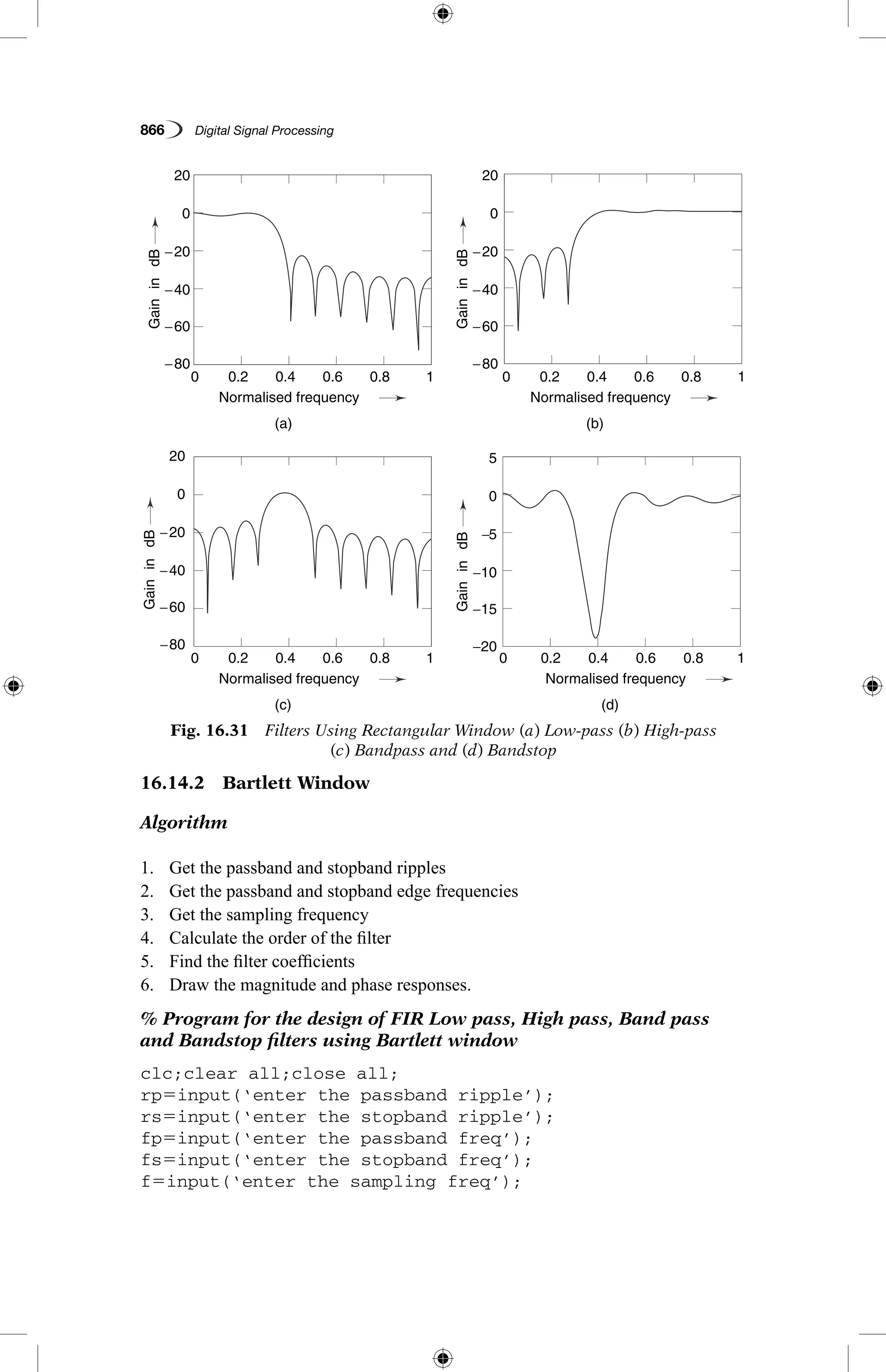
The gain responses of low-pass, high-pass, bandpass and bandstop filters using
rectangular window are shown in Fig. 16.31.](https://image.slidesharecdn.com/matlabprograms-150130053105-conversion-gate01/75/Matlab-programs-51-2048.jpg)
![MATLAB Programs 867
wp52*fp/f;ws52*fs/f;
num5220*log10(sqrt(rp*rs))213;
dem514.6*(fs2fp)/f;
n5ceil(num/dem);
n15n11;
if (rem(n,2)˜50)
n15n;
n5n21;
end
y5bartlett(n1);
% low-pass filter
b5fir1(n,wp,y);
[h,o]5freqz(b,1,256);
m520*log10(abs(h));
subplot(2,2,1);plot(o/pi,m);ylabel(‘Gain in dB --.’);
xlabel(‘(a) Normalised frequency --.’);
% high-pass filter
b5fir1(n,wp,’high’,y);
[h,o]5freqz(b,1,256);
m520*log10(abs(h));
subplot(2,2,2);plot(o/pi,m);ylabel(‘Gain in dB --.’);
xlabel(‘(b) Normalised frequency --.’);
% band pass filter
wn5[wp ws];
b5fir1(n,wn,y);
[h,o]5freqz(b,1,256);
m520*log10(abs(h));
subplot(2,2,3);plot(o/pi,m);ylabel(‘Gain in dB --.’);
xlabel(‘(c) Normalised frequency --.’);
% band stop filter
b5fir1(n,wn,’stop’,y);
[h,o]5freqz(b,1,256);
m520*log10(abs(h));
subplot(2,2,4);plot(o/pi,m);ylabel(‘Gain in dB --.’);
xlabel(‘(d) Normalised frequency --.’);
As an example,
enter the passband ripple 0.04
enter the stopband ripple 0.02
enter the passband freq 1500
enter the stopband freq 2000
enter the sampling freq 8000
The gain responses of low-pass, high-pass, bandpass and bandstop filters using
Bartlett window are shown in Fig. 16.32.](https://image.slidesharecdn.com/matlabprograms-150130053105-conversion-gate01/75/Matlab-programs-53-2048.jpg)
![MATLAB Programs 869
wp52*fp/f;ws52*fs/f;
num5220*log10(sqrt(rp*rs))213;
dem514.6*(fs2fp)/f;
n5ceil(num/dem);
n15n11;
if (rem(n,2)˜50)
n15n;
n5n21;
end
y5blackman(n1);
% low-pass filter
b5fir1(n,wp,y);
[h,o]5freqz(b,1,256);
m520*log10(abs(h));
subplot(2,2,1);plot(o/pi,m);ylabel(‘Gain in dB --.’);
xlabel(‘(a) Normalised frequency --.’);
% high-pass filter
b5fir1(n,wp,’high’,y);
[h,o]5freqz(b,1,256);
m520*log10(abs(h));
subplot(2,2,2);plot(o/pi,m);ylabel(‘Gain in dB --.’);
xlabel(‘(b) Normalised frequency --.’);
% band pass filter
wn5[wp ws];
b5fir1(n,wn,y);
[h,o]5freqz(b,1,256);
m520*log10(abs(h));
subplot(2,2,3);plot(o/pi,m);ylabel(‘Gain in dB --.’);
xlabel(‘(c) Normalised frequency --.’);
% band stop filter
b5fir1(n,wn,’stop’,y);
[h,o]5freqz(b,1,256);
m520*log10(abs(h));
subplot(2,2,4);plot(o/pi,m);;ylabel(‘Gain in dB --.’);
xlabel(‘(d) Normalised frequency --.’);
As an example,
enter the passband ripple 0.03
enter the stopband ripple 0.01
enter the passband freq 2000
enter the stopband freq 2500
enter the sampling freq 7000
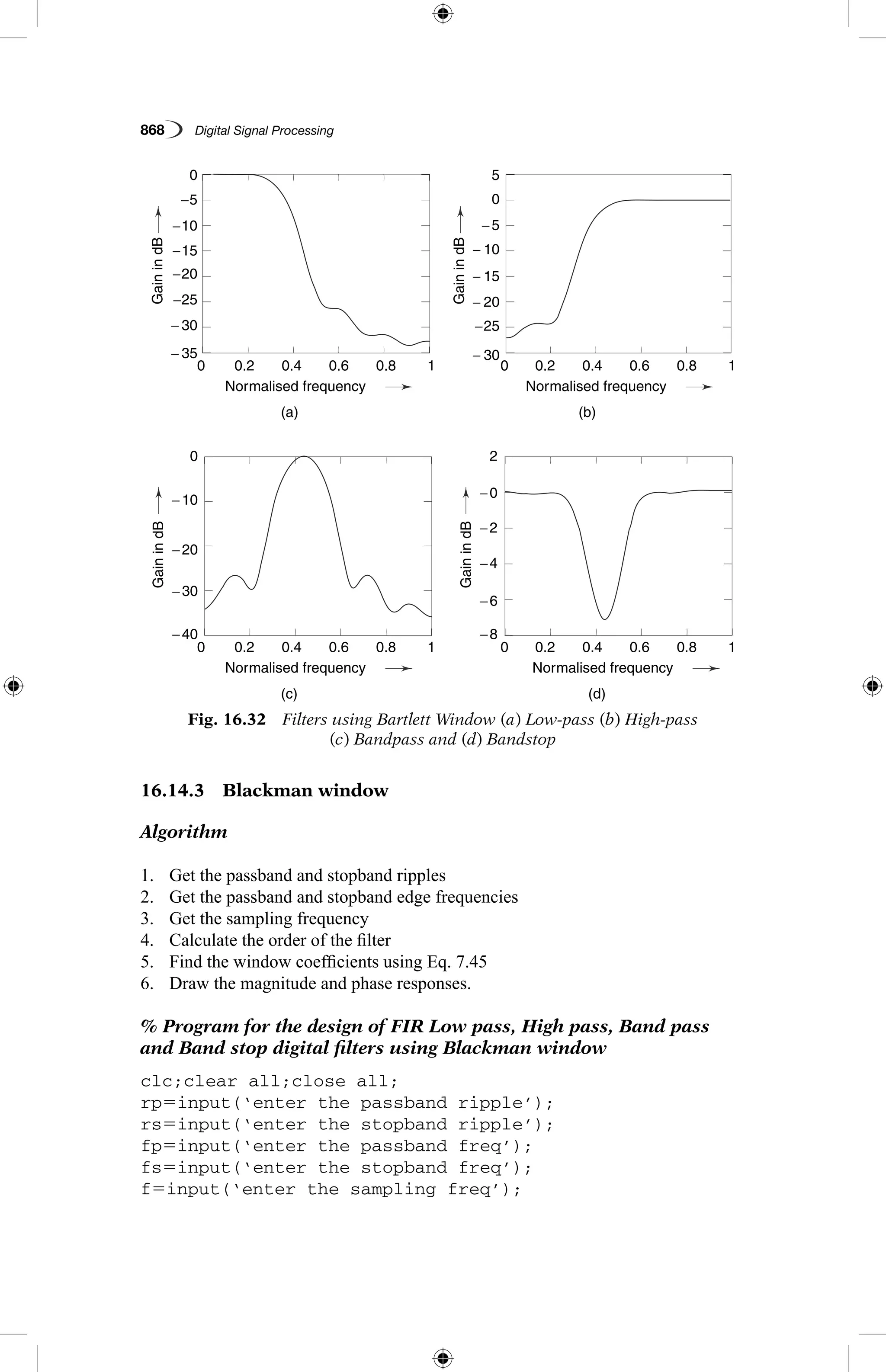
The gain responses of low-pass, high-pass, bandpass and bandstop filters using
Blackman window are shown in Fig. 16.33.](https://image.slidesharecdn.com/matlabprograms-150130053105-conversion-gate01/75/Matlab-programs-55-2048.jpg)

![MATLAB Programs 871
r5input(‘enter the ripple value(in dBs)’);
wp52*fp/f;ws52*fs/f;
num5220*log10(sqrt(rp*rs))213;
dem514.6*(fs2fp)/f;
n5ceil(num/dem);
if(rem(n,2)˜50)
n5n11;
end
y5chebwin(n,r);
% low-pass filter
b5fir1(n-1,wp,y);
[h,o]5freqz(b,1,256);
m520*log10(abs(h));
subplot(2,2,1);plot(o/pi,m);ylabel(‘Gain in dB --.’);
xlabel(‘(a) Normalised frequency --.’);
% high-pass filter
b5fir1(n21,wp,’high’,y);
[h,o]5freqz(b,1,256);
m520*log10(abs(h));
subplot(2,2,2);plot(o/pi,m);ylabel(‘Gain in dB --.’);
xlabel(‘(b) Normalised frequency --.’);
% band-pass filter
wn5[wp ws];
b5fir1(n21,wn,y);
[h,o]5freqz(b,1,256);
m520*log10(abs(h));
subplot(2,2,3);plot(o/pi,m);ylabel(‘Gain in dB --.’);
xlabel(‘(c) Normalised frequency --.’);
% band-stop filter
b5fir1(n21,wn,’stop’,y);
[h,o]5freqz(b,1,256);
m520*log10(abs(h));
subplot(2,2,4);plot(o/pi,m);ylabel(‘Gain in dB --.’);
xlabel(‘(d) Normalised frequency --.’);
As an example,
enter the passband ripple 0.03
enter the stopband ripple 0.02
enter the passband freq 1800
enter the stopband freq 2400
enter the sampling freq 10000
enter the ripple value(in dBs)40
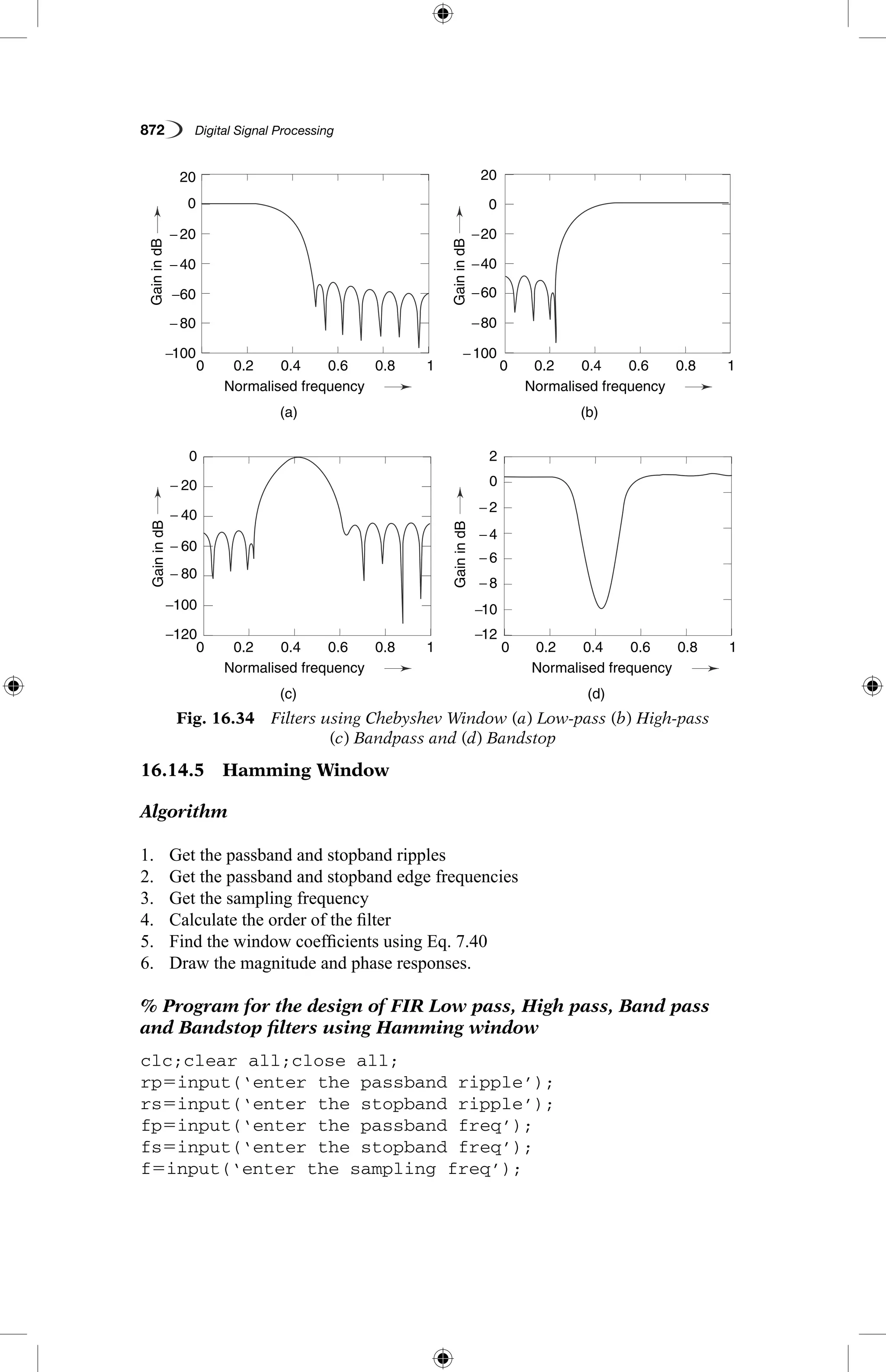
The gain responses of low-pass, high-pass, bandpass and bandstop filters using
Chebyshev window are shown in Fig. 16.34.](https://image.slidesharecdn.com/matlabprograms-150130053105-conversion-gate01/75/Matlab-programs-57-2048.jpg)
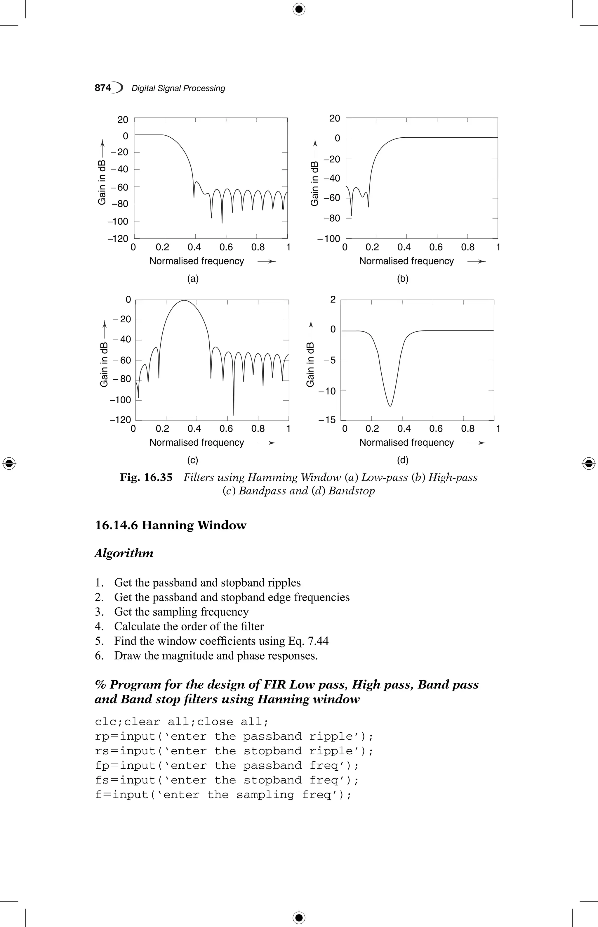
![MATLAB Programs 873
wp52*fp/f;ws52*fs/f;
num5220*log10(sqrt(rp*rs))213;
dem514.6*(fs2fp)/f;
n5ceil(num/dem);
n15n11;
if (rem(n,2)˜50)
n15n;
n5n21;
end
y5hamming(n1);
% low-pass filter
b5fir1(n,wp,y);
[h,o]5freqz(b,1,256);
m520*log10(abs(h));
subplot(2,2,1);plot(o/pi,m);ylabel(‘Gain in dB --.’);
xlabel(‘(a) Normalised frequency --.’);
% high-pass filter
b5fir1(n,wp,’high’,y);
[h,o]5freqz(b,1,256);
m520*log10(abs(h));
subplot(2,2,2);plot(o/pi,m);ylabel(‘Gain in dB --.’);
xlabel(‘(b) Normalised frequency --.’);
% band pass filter
wn5[wp ws];
b5fir1(n,wn,y);
[h,o]5freqz(b,1,256);
m520*log10(abs(h));
subplot(2,2,3);plot(o/pi,m);ylabel(‘Gain in dB --.’);
xlabel(‘(c) Normalised frequency --.’);
% band stop filter
b5fir1(n,wn,’stop’,y);
[h,o]5freqz(b,1,256);
m520*log10(abs(h));
subplot(2,2,4);plot(o/pi,m);ylabel(‘Gain in dB --.’);
xlabel(‘(d) Normalised frequency --.’);
As an example,
enter the passband ripple 0.02
enter the stopband ripple 0.01
enter the passband freq 1200
enter the stopband freq 1700
enter the sampling freq 9000
The gain responses of low-pass, high-pass, bandpass and bandstop filters using
Hamming window are shown in Fig. 16.35.](https://image.slidesharecdn.com/matlabprograms-150130053105-conversion-gate01/75/Matlab-programs-59-2048.jpg)
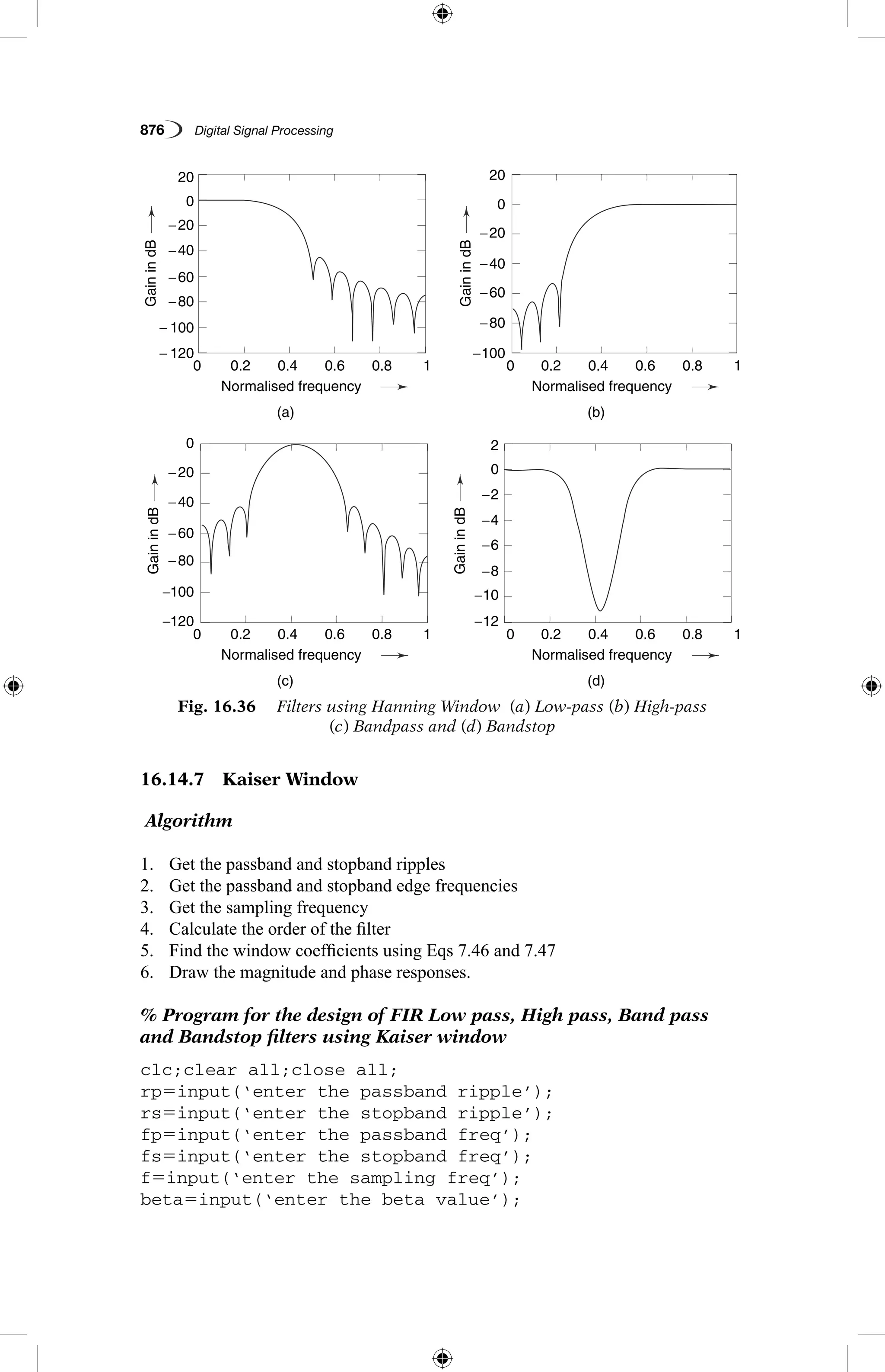
![MATLAB Programs 875
wp52*fp/f;ws52*fs/f;
num5220*log10(sqrt(rp*rs))213;
dem514.6*(fs2fp)/f;
n5ceil(num/dem);
n15n11;
if (rem(n,2)˜50)
n15n;
n5n21;
end
y5hamming(n1);
% low-pass filter
b5fir1(n,wp,y);
[h,o]5freqz(b,1,256);
m520*log10(abs(h));
subplot(2,2,1);plot(o/pi,m);ylabel(‘Gain in dB --.’);
xlabel(‘(a) Normalised frequency --.’);
% high-pass filter
b5fir1(n,wp,’high’,y);
[h,o]5freqz(b,1,256);
m520*log10(abs(h));
subplot(2,2,2);plot(o/pi,m);ylabel(‘Gain in dB --.’);
xlabel(‘(b) Normalised frequency --.’);
% band pass filter
wn5[wp ws];
b5fir1(n,wn,y);
[h,o]5freqz(b,1,256);
m520*log10(abs(h));
subplot(2,2,3);plot(o/pi,m);ylabel(‘Gain in dB --.’);
xlabel(‘(c) Normalised frequency --.’);
% band stop filter
b5fir1(n,wn,’stop’,y);
[h,o]5freqz(b,1,256);
m520*log10(abs(h));
subplot(2,2,4);plot(o/pi,m);ylabel(‘Gain in dB --.’);
xlabel(‘(d) Normalised frequency --.’);
As an example,
enter the passband ripple 0.03
enter the stopband ripple 0.01
enter the passband freq 1400
enter the stopband freq 2000
enter the sampling freq 8000
The gain responses of low-pass, high-pass, bandpass and bandstop filters using
Hanning window are shown in Fig. 16.36.](https://image.slidesharecdn.com/matlabprograms-150130053105-conversion-gate01/75/Matlab-programs-61-2048.jpg)
![MATLAB Programs 877
wp52*fp/f;ws52*fs/f;
num5220*log10(sqrt(rp*rs))213;
dem514.6*(fs2fp)/f;
n5ceil(num/dem);
n15n11;
if (rem(n,2)˜50)
n15n;
n5n21;
end
y5kaiser(n1,beta);
% low-pass filter
b5fir1(n,wp,y);
[h,o]5freqz(b,1,256);
m520*log10(abs(h));
subplot(2,2,1);plot(o/pi,m);ylabel(‘Gain in dB --’);
xlabel(‘(a) Normalised frequency --’);
% high-pass filter
b5fir1(n,wp,’high’,y);
[h,o]5freqz(b,1,256);
m520*log10(abs(h));
subplot(2,2,2);plot(o/pi,m);ylabel(‘Gain in dB --’);
xlabel(‘(b) Normalised frequency --’);
% band pass filter
wn5[wp ws];
b5fir1(n,wn,y);
[h,o]5freqz(b,1,256);
m520*log10(abs(h));
subplot(2,2,3);plot(o/pi,m);ylabel(‘Gain in dB --’);
xlabel(‘(c) Normalised frequency --’);
% band stop filter
b5fir1(n,wn,’stop’,y);
[h,o]5freqz(b,1,256);
m520*log10(abs(h));
subplot(2,2,4);plot(o/pi,m);ylabel(‘Gain in dB --’);
xlabel(‘(d) Normalised frequency --’);
As an example,
enter the passband ripple 0.02
enter the stopband ripple 0.01
enter the passband freq 1000
enter the stopband freq 1500
enter the sampling freq 10000
enter the beta value 5.8
The gain responses of low-pass, high-pass, bandpass and bandstop filters using
Kaiser window are shown in Fig. 16.37.](https://image.slidesharecdn.com/matlabprograms-150130053105-conversion-gate01/75/Matlab-programs-63-2048.jpg)
![878 Digital Signal Processing
16.15 UPSAMPLING A SINUSOIDAL SIGNAL
% Program for upsampling a sinusoidal signal by factor L
N5input(‘Input length of the sinusoidal sequence5’);
L5input(‘Up Samping factor5’);
fi5input(‘Input signal frequency5’);
% Generate the sinusoidal sequence for the specified length N
n50:N21;
x5sin(2*pi*fi*n);
% Generate the upsampled signal
y5zeros (1,L*length(x));
y([1:L:length(y)])5x;
%Plot the input sequence
subplot (2,1,1);
stem (n,x);
title(‘Input Sequence’);
xlabel(‘Time n’);
ylabel(‘Amplitude’);
Fig. 16.37 Filters using Kaiser Window (a) Low-pass (b) High-pass
(c) Bandpass and (d) Bandstop
−120
−120 −15
−40
−20
−60
−80
−100
−100
−10
−5
0
−80
− 60
− 80
− 40
− 20
− 60
− 40
− 20
0
20
0
0 5
20
0.2
0.2
0.2
0.2
0.4
0.4
0.4
0.4
(a)
(c)
(b)
(d)
Normalised frequency
Normalised frequency
Normalised frequency
Normalised frequency
0.6
0.6
0.6
0.6
0.8
0.8
0.8
0.8
1
1
1
1
0
0
0
0
GainindB
GainindB
GainindB
GainindB](https://image.slidesharecdn.com/matlabprograms-150130053105-conversion-gate01/75/Matlab-programs-64-2048.jpg)
![MATLAB Programs 879
%Plot the output sequence
subplot (2,1,2);
stem (n,y(1:length(x)));
title(‘[output sequence,upsampling factor5‘,num2str(L)]);
xlabel(‘Time n’);
ylabel(‘Amplitude’);
16.16
UPSAMPLING AN EXPONENTIAL
SEQUENCE
% Program for upsampling an exponential sequence by a factor M
n5input(‘enter length of input sequence …’);
l5input(‘enter up sampling factor …’);
% Generate the exponential sequence
m50:n21;
a5input(‘enter the value of a …’);
x5a.^m;
% Generate the upsampled signal
y5zeros(1,l*length(x));
y([1:l:length(y)])5x;
figure(1)
stem(m,x);
xlabel({‘Time n’;’(a)’});
ylabel(‘Amplitude’);
figure(2)
stem(m,y(1:length(x)));
xlabel({‘Time n’;’(b)’});
ylabel(‘Amplitude’);
As an example,
enter length of input sentence … 25
enter upsampling factor … 3
enter the value of a … 0.95
The input and output sequences of upsampling an exponential sequence an
are shown
in Fig. 16.38.
Fig. 16.38 (Contd.)](https://image.slidesharecdn.com/matlabprograms-150130053105-conversion-gate01/75/Matlab-programs-65-2048.jpg)
![880 Digital Signal Processing
16.17
DOWN SAMPLING A SINUSOIDAL
SEQUENCE
% Program for down sampling a sinusoidal sequence by a factor M
N5input(‘Input length of the sinusoidal signal5’);
M5input(‘Down samping factor5’);
fi5input(‘Input signal frequency5’);
%Generate the sinusoidal sequence
n50:N21;
m50:N*M21;
x5sin(2*pi*fi*m);
%Generate the down sampled signal
y5x([1:M:length(x)]);
%Plot the input sequence
subplot (2,1,1);
stem(n,x(1:N));
title(‘Input Sequence’);
xlabel(‘Time n’);
ylabel(‘Amplitude’);
%Plot the down sampled signal sequence
subplot(2,1,2);
stem(n,y);
title([‘Outputsequencedownsamplingfactor’,num2str(M)]);
xlabel(‘Time n’);
ylabel(‘Amplitude’);
16.18
DOWN SAMPLING AN EXPONENTIAL
SEQUENCE
% Program for downsampling an exponential sequence by a factor M
N5input(‘enter the length of the output sequence …’);
M5input(‘enter the down sampling factor …’);
Fig. 16.38 (a) Input Exponential Sequence
(b) Output Sequence Upsampled by a Factor of 3](https://image.slidesharecdn.com/matlabprograms-150130053105-conversion-gate01/75/Matlab-programs-66-2048.jpg)
![MATLAB Programs 881
% Generate the exponential sequence
n50:N21;
m50:N*M21;
a5input(‘enter the value of a …’);
x5a.^m;
% Generate the downsampled signal
y5x([1:M:length(x)]);
figure(1)
stem(n,x(1:N));
xlabel({‘Time n’;’(a)’});
ylabel(‘Amplitude’);
figure(2)
stem(n,y);
xlabel({‘Time n’;’(b)’});
ylabel(‘Amplitude’);
As an example,
enter the length of the output sentence … 25
enter the downsampling factor … 3
enter the value of a … 0.95
The input and output sequences of downsampling an exponential sequence an
are
shown in Fig. 16.39.
Fig. 16.39 (a) Input Exponential Sequence
(b) Output Sequence Downsampled by a Factor of 3](https://image.slidesharecdn.com/matlabprograms-150130053105-conversion-gate01/75/Matlab-programs-67-2048.jpg)
![882 Digital Signal Processing
16.19 DECIMATOR
% Program for downsampling the sum of two sinusoids using
MATLAB’s inbuilt decimation function by a factor M
N5input(‘Length of the input signal5’);
M5input(‘Down samping factor5’);
f15input(‘Frequency of first sinusoid5’);
f25input(‘Frequency of second sinusoid5’);
n50:N21;
% Generate the input sequence
x52*sin(2*pi*f1*n)13*sin(2*pi*f2*n);
%Generate the decimated signal
% FIR low pass decimation is used
y5decimate(x,M,‘fir’);
%Plot the input sequence
subplot (2,1,1);
stem (n,x(1:N));
title(‘Input Sequence’);
xlabel(‘Time n’);
ylabel(‘Amplitude’);
%Plot the output sequence
subplot (2,1,2);
m50:N/M21;
stem (m,y(1:N/M));
title([‘Outputsequencedownsamplingfactor’,num2str(M)]);
xlabel(‘Time n’);
ylabel(‘Amplitude’);
16.20 DECIMATOR AND INTERPOLATOR
% Program for downsampling and upsampling the sum of two
sinusoids using MATLAB’s inbuilt decimation and interpolation
function by a factor of 20.
%Generate the input sequence for Fs
5200Hz, f1
550Hz and
f2
5100 Hz
t50:1/200:10;
y53.*cos(2*pi*50.*t/200)11.*cos(2*pi*100.*t/200);
figure(1)
stem(y);
xlabel({‘Times in Seconds’;’(a)});
ylabel(‘Amplitude’);](https://image.slidesharecdn.com/matlabprograms-150130053105-conversion-gate01/75/Matlab-programs-68-2048.jpg)
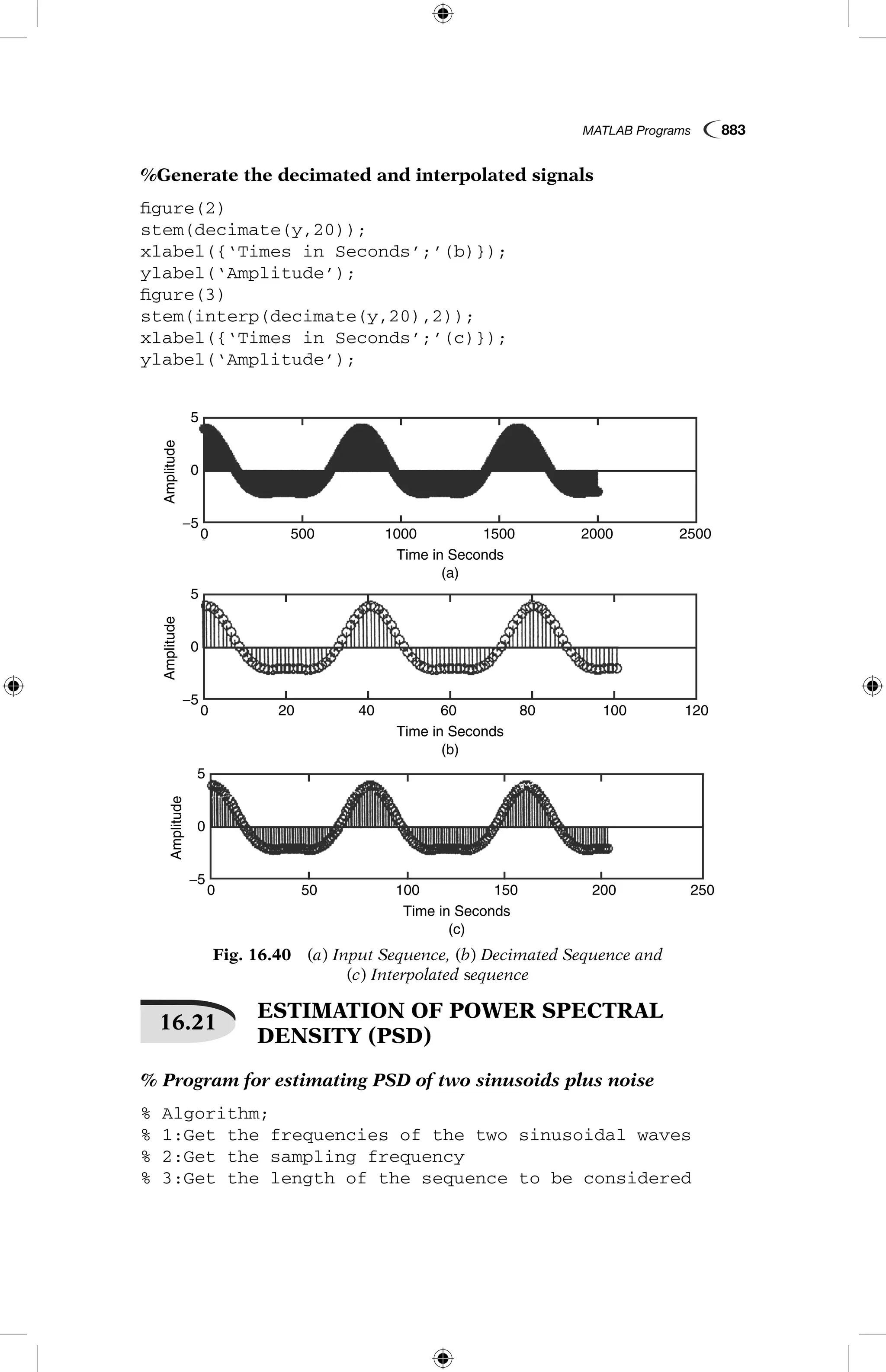
![884 Digital Signal Processing
% 4:Get the two FFT lengths for comparing the corre-
sponding power spectral densities
clc; close all; clear all;
f15input(‘Enter the frequency of first sinusoid’);
f25input(‘Enter the frequency of second sinusoid’);
fs5input(‘Enter the sampling frequency’);
N5input(“Enter the length of the input sequence’);
N15input(“Enter the input FFT length 1’);
N25input(“Enter the input FFT length 2’);
%Generation of input sequence
t50:1/fs:1;
x52*sin(2*pi*f1*1)13*sin(2*pi*f2*t)2randn(size(t));
%Generation of psd for two different FFT lengths
Pxx15abs(fft(x,N1)).^2/(N11);
Pxx25abs(fft(x,N2)).^2/(N11);
%Plot the psd;
subplot(2,1,1);
plot ((0:(N121))/N1*fs,10*log10(Pxx1));
xlabel(‘Frequency in Hz’);
ylabel(‘Power spectrum in dB’);
title(‘[PSD with FFT length,num2str(N1)]’);
subplot (2,1,2);
plot ((0:(N221))/N2*fs,10*log10(Pxx2));
xlabel(‘Frequency in Hz’);
ylabel(‘Power spectrum in dB’);
title(‘[PSD with FFT length,num2str(N2)]’);
16.22 PSD ESTIMATOR
% Program for estimating PSD of a two sinusoids plus noise using
%(i)non-overlapping sections
%(ii)overlapping sections and averaging the periodograms
clc; close all; clear all;
f15input(‘Enter the frequency of first sinusoid’);
f25input(‘Enter the frequency of second sinusoid’);
fs5input(‘Enter the sampling frequency’);
N5input(“Enter the length of the input sequence’);
N15input(“Enter the input FFT length 1’);
N25input(“Enter the input FFT length 2’);
%Generation of input sequence
t50:1/fs:1;
x52*sin(2*pi*f1*1)13*sin(2*pi*f2*t)2randn(size(t));](https://image.slidesharecdn.com/matlabprograms-150130053105-conversion-gate01/75/Matlab-programs-70-2048.jpg)
![MATLAB Programs 885
%Generation of psd for two different FFT lengths
Pxx15(abs(fft(x(1:256))).^21abs(fft(x(257:512))).^21
abs(fft(x(513:768))).^2/(256*3); %using nonoverlapping
sections
Pxx25(abs(fft(x(1:256))).^21abs(fft(x(129:384))).^21ab
s(fft(x(257:512))).^21abs(fft(x(385:640))).^21abs(fft(
x(513:768))).^21abs(fft(x(641:896))).^2/(256*6); %using
overlapping sections
% Plot the psd;
subplot (2,1,1);
plot ((0:255)/256*fs,10*log10(Pxx1));
xlabel(‘Frequency in Hz’);
ylabel(‘Power spectrum in dB’);
title(‘[PSD with FFT length,num2str(N1)]’);
subplot (2,1,2);
plot ((0:255)/256*fs,10*log10(Pxx2));
xlabel(‘Frequency in Hz’);
ylabel(‘Power spectrum in dB’);
title(‘[PSD with FFT length,num2str(N2)]’);
16.23 PERIODOGRAM ESTIMATION
% Periodogram estimate cold be done by applying a non-
rectangular data windows to the sections prior to com-
puting the periodogram
% This program estimates PSD for the input signal of two
sinusoids plus noise using Hanning window
f15input(‘Enter the frequency of first sinusoid’);
f25input(‘Enter the frequency of second sinusoid’);
fs5input(‘Enter the sampling frequency’);
t50:1/fs:1;
w5hanning(256);
x52*sin(2*pi*f1*t)13*sin(2*pi*f2*t)2randn(size(t));
Pxx5(abs(fft(w.*x(1:256))).^21abs(fft(w.*x(129:384))).^
21abs(fft(w.*x(257:512))).^21abs(fft(w.*x(385:640))).^2
1abs(fft(w.*x(513:768))).^21abs(fft(w.*x(641:896))).^2/
(norm(w)^2*6);
Plot((0:255)/256*fs,10*log10(Pxx));
16.24 WELCH PSD ESTIMATOR
% Program for estimating the PSD of sum of two sinusoids plus
noise using Welch method
n50.01:0.001:.1;
x5sin(.25*pi*n)13*sin(.45*pi*n)1rand(size(n));
pwelch(x)](https://image.slidesharecdn.com/matlabprograms-150130053105-conversion-gate01/75/Matlab-programs-71-2048.jpg)
![886 Digital Signal Processing
xlabel(‘Normalised Frequency (x pi rad/sample)’);
ylabel(‘Power Spectrum Density (dB/rad/sample)’)
16.25 WELCH PSD ESTIMATOR USING WINDOWS
% Program for estimating the PSD of sum of two sinusoids using
Welch method with an overlap of 50 percent and with Hanning,
Hamming, Bartlett, Blackman and rectangular windows.
fs51000;
t50:1/fs:3;
x5sin(2*pi*200*t)1sin(2*pi*400*t);
figure(1)
subplot(211)
pwelch(x,[],[],[],fs);
title(‘Overlay plot of 50 Welch estimates’)
subplot(212)
pwelch(x,hanning(512),0,512,fs)
title(‘N5512 Overlap550% Hanning’)
figure(2)
subplot(211)
pwelch(x,[],[],[],fs);
title(‘Overlay plot of 50 Welch estimates’)
subplot(212)
pwelch(x,hamming(512),0,512,fs)
title(‘N5512 Overlap550% Hamming’)
figure(3)
subplot(211)
pwelch(x,[],[],[],fs);
title(‘Overlay plot of 50 Welch estimates’)
subplot(212)
pwelch(x,bartlett(512),0,512,fs)
title(‘N5512 Overlap550% Bartlett’)
figure(4)
subplot(211)
pwelch(x,[],[],[],fs);
Fig. 16.41 Welch PSD Estimate
5
0
−5
−10
−15
−20
0 0.1 0.2 0.3 0.4 0.5
Welch PSD Estimate
PowerSpectrumDensity(dB/rad/sample)
Normalised Frequency (x pi rad/sample)
0.6 0.7 0.8 0.9 1](https://image.slidesharecdn.com/matlabprograms-150130053105-conversion-gate01/75/Matlab-programs-72-2048.jpg)
![MATLAB Programs 887
Fig. 16.42 (b) Welch Estimate with N5512, 50% Overlap Hamming
0
−20
−40
−60
0 50 100 150 200
Frequency (Hz)
Overlay plot of 50 Welch estimates
PowerSpectralDensity(dB/Hz)
250 300 350 400 450 500
−80
0
−20
−40
−60
0 50 100 150 200
Frequency (Hz)
N=512 Overlap = 50% Hamming
PowerSpectralDensity(dB/Hz)
250 300 350 400 450 500
−80
0
−20
−40
−60
0 50 100 150 200
Frequency (Hz)
N=512 Overlap = 50% Hanning
Overlay plot of 50 Welch estimates
PowerSpectralDensity(dB/Hz)
250 300 350 400 450 500
0 50 100 150 200
Frequency (Hz)
250 300 350 400 450 500
−80
0
−50
−100
PowerSpectralDensity(dB/Hz)
−150
Fig. 16.42 (a) Welch Estimate with N5512, 50% Overlap Hanning
title(‘Overlay plot of 50 Welch estimates’)
subplot(212)
pwelch(x,blackman(512),0,512,fs)
title(‘N5512 Overlap550% Blackman’)
figure(5)
subplot(211)
pwelch(x,[],[],[],fs);
title(‘Overlay plot of 50 Welch estimates’)
subplot(212)
pwelch(x,boxcar(512),0,512,fs)
title(‘N5512 Overlap550% Rectangular’)](https://image.slidesharecdn.com/matlabprograms-150130053105-conversion-gate01/75/Matlab-programs-73-2048.jpg)
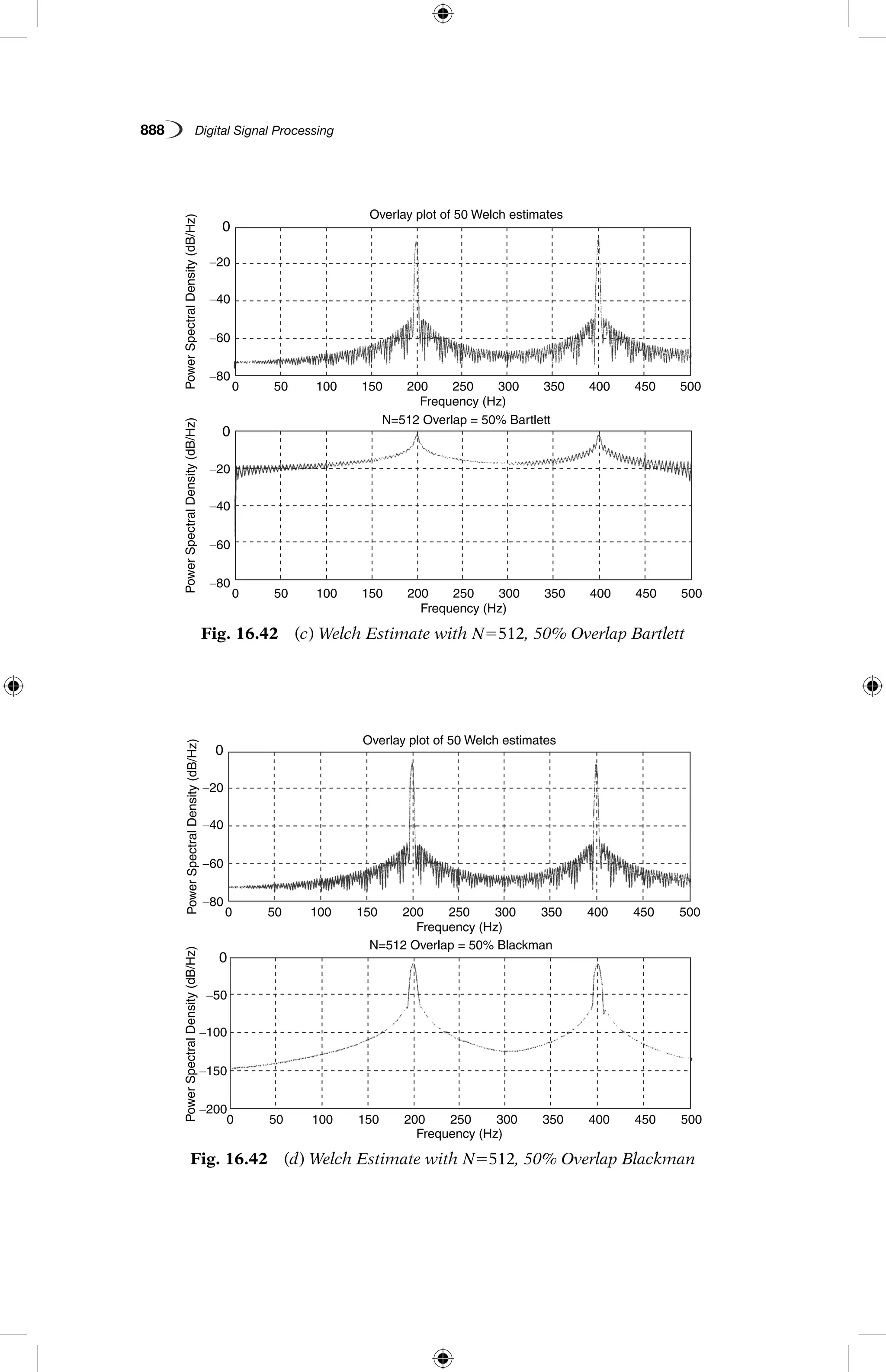
![MATLAB Programs 889
Fig. 16.42 (e) Welch Estimate with N5512, 50% Overlap Rectangular
0
−20
−40
−60
0 50 100 150 200
Frequency (Hz)
Overlay plot of 50 Welch estimates
PowerSpectralDensity(dB/Hz)
250 300 350 400 450 500
−80
0
−10
−20
−30
−40
−50
−60
0 50 100 150 200
Frequency (Hz)
N = 512 Overlap = 50% Rectangular
PowerSpectralDensity(dB/Hz)
250 300 350 400 450 500
16.26 WELCH PSD ESTIMATOR USING WINDOWS
% Program for estimating the PSD of sum of two sinusoids plus
noise using Welch method with an overlap of 50 percent and with
Hanning, Hamming, Bartlett, Blackman and rectangular windows
fs51000;
t50:1/fs:3;
x52*sin(2*pi*200*t)15*sin(2*pi*400*t);
y5x1randn(size(t));
figure(1)
subplot(211);
pwelch(y,[],[],[],fs);
title(‘Overlay plot of 50 Welch estimates’);
subplot(212);
pwelch(y,hanning(512),0,512,fs);
title(‘N5512 Overlap550% Hanning’);
figure(2)
subplot(211);
pwelch(y,[],[],[],fs);
title(‘Overlay plot of 50 Welch estimates’);
subplot(212);
pwelch(y,hamming(512),0,512,fs);
title(‘N5512 Overlap550% Hamming’);](https://image.slidesharecdn.com/matlabprograms-150130053105-conversion-gate01/75/Matlab-programs-75-2048.jpg)
![890 Digital Signal Processing
10
0
−10
−20
−30
0 50 100 150 200
Overlay plot of 50 Welch estimates
Frequency (Hz)
PowerSpectralDensity(dB/Hz)
250 300 350 400 450 500
−40
10
0
−10
−20
−30
0 50 100 150 200
N=512 Overlap = 50% Hanning
Frequency (Hz)
PowerSpectralDensity(dB/Hz)
250 300 350 400 450 500
−40
Fig. 16.43 (a) Welch Estimate with N5512, 50% Overlap Hanning
figure(3)
subplot(211);
pwelch(y,[],[],[],fs);
title(‘Overlay plot of 50 Welch estimates’);
subplot(212);
pwelch(y,bartlett(512),0,512,fs);
title(‘N5512 Overlap550% Bartlett’);
figure(4)
subplot(211);
pwelch(y,[],[],[],fs);
title(‘Overlay plot of 50 Welch estimates’);
subplot(212);
pwelch(y,blackman(512),0,512,fs);
title(‘N5512 Overlap550% Blackman’);
figure(5)
subplot(211);
pwelch(y,[],[],[],fs);
title(‘Overlay plot of 50 Welch estimates’);
subplot(212);
pwelch(y,boxcar(512),0,512,fs);
title(‘N5512 Overlap550% Rectangular’);](https://image.slidesharecdn.com/matlabprograms-150130053105-conversion-gate01/75/Matlab-programs-76-2048.jpg)
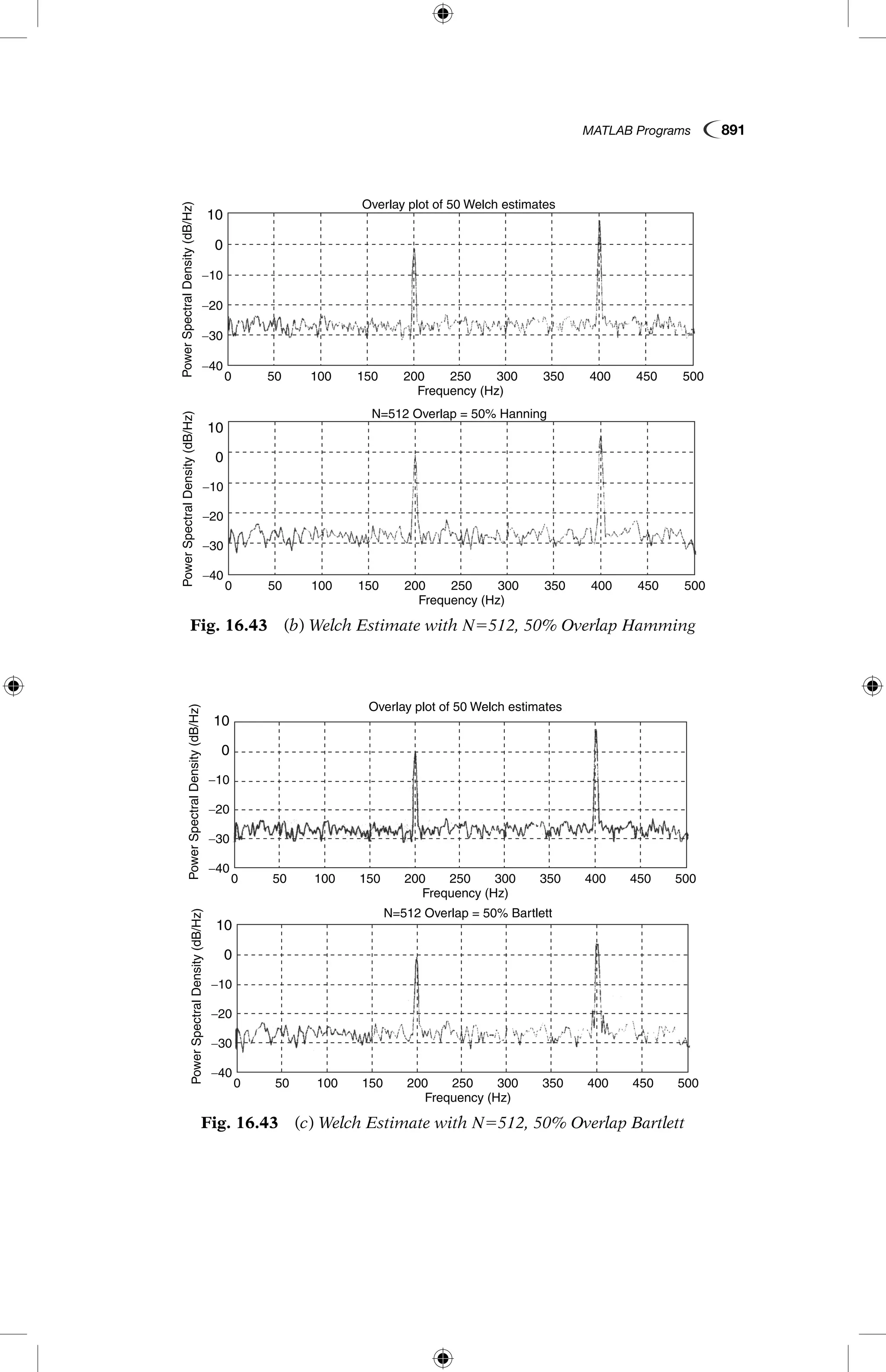
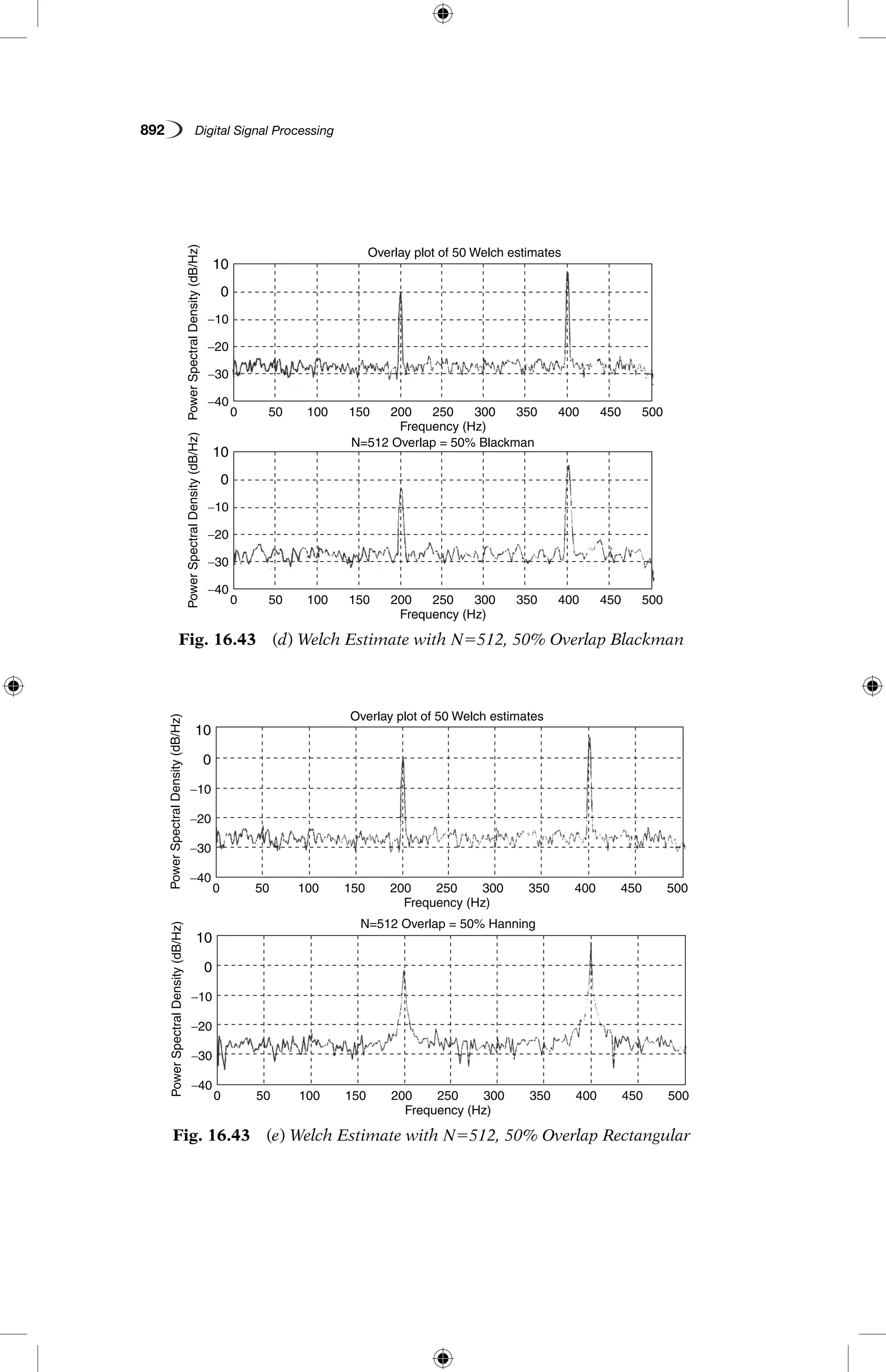
![MATLAB Programs 893
16.27 STATE-SPACE REPRESENTATION
% Program for computing the state-space matrices from the given
transfer function
function [A,B,C,D]5tf2ss(b,a);
a5input (‘enter the denominator polynomials5’);
b5input (‘enter the numerator polynomials5’);
p5length(a)21;q5length(b)21;N5max(p,q);
if(Np),a5[a,zeros(1,N2p)];end
if(Nq),b5[b,zeros(1,N2q)];end
A5[2a(2:N11);[eye(N21),zeros(N21,1)]];
B5[1;zeros(N21,1)];
C5b(2:N11)2b(1)*(2:N11);
D5b(1);
16.28 PARTIAL FRACTION DECOMPOSITION
% Program for partial fraction decomposition of a rational transfer
function
function[c,A,alpha]5tf2pf(b,a);
a5input (‘enter the denominator polynomials5’);
b5input (‘enter the numerator polynomials5’);
p5length(a)21;
q5length(b)21;
a5(1/a(1))*reshape(a,1,p11);
b5(1/a(1))*reshape(b,1,q11);
if(q5p),%case of nonempty c(z)
temp5toeplitz([a,zeros(1,q2p)]’,[a(1),zeros(1,q2p)]);
temp5[temp,[eye(p);zeros(q2p11,p)]);
temp5temp/b’;
c5temp(1:;q2p11);
d5temp(q2p12:q11)’;
else
c5[];
d5[b,zeros(1,p2q21)];
end
alpha5cplxpair (roots(a));’;
A5zeros(1,p);
for k51 :p
temp5prod(alpha(k)2alpha(find(1:p5k)));
if(temp550),error(‘repeated roots in TF2PF’);
else,A(k)5polyval(d,alpha(k))/temp;
end
end](https://image.slidesharecdn.com/matlabprograms-150130053105-conversion-gate01/75/Matlab-programs-79-2048.jpg)
![894 Digital Signal Processing
16.29 INVERSE z-TRANSFORM
% Program for computing inverse z-transform of a rational transfer
function
function x5invz(b,a,N);
b5input (‘enter the numerator polynomials5’);
a5input (‘enter the denominator polynomials5’);
N5input (‘enter the number of points to be computed5’);
[c,A,alpha]5tf2pf(b,a);
x5zeros (1,N);
x(1:length(c))5c;
for k51:length(A),
x5x1A(k)*(alpha(k)).^(0:N21);
end
x5real(x);
16.30 GROUP DELAY
% Program for computing group delay of a rational transfer
function on a given frequency interval
function D5grpdly(b,a,K,theta);
b5input (‘enter the numerator polynomials5’);
a5input (‘enter the denominator polynomials5’);
K5input (‘enter the number of frequency response
points5’);
theta5input (‘enter the theta value5’);
a5reshape(a,1,length(a));
b5reshape(b,1,length(b));
if (length(a)551)%case of FIR
bd52j*(0:length(b)21).*b;
if(nargin553),
B5frqresp(b,1,K);
Bd5frqresp(bd,1,K);
else,
B5frqresp(b,1,K,theta);
Bd5frqresp(bd,1,K,theta);
end
D5(real(Bd).*imag(B)2real(B).*imag(Bd))./abs(B).^2;
else %case of IIR
if(nargin553),
D5grpdly (b,1,K)2grpdly(a,1,K);
else,
D5grpdly(b,1,K,theta)2grpdly(a,1,K,theta);
end
end](https://image.slidesharecdn.com/matlabprograms-150130053105-conversion-gate01/75/Matlab-programs-80-2048.jpg)
![MATLAB Programs 895
16.31
IIR FILTER DESIGN-IMPULSE INVARIANT
METHOD
% Program for transforming an analog filter into a digital filter using
impulse invariant technique
function [bout,aout]5impinv(bin,ain,T);
bin5input(‘enter the numerator polynomials5’);
ain5input(‘enter the denominator polynomials5’);
T5input(‘enter the sampling interval5’);
if(length(bin)5length(ain)),
error(‘Anlog filter in IMPINV is not strictly proper’);
end
[r,p,k]5residue(bin,ain);
[bout,aout]5pf2tf([],T*r,exp(T*p));
16.32
IIR FILTER DESIGN-BILINEAR
TRANSFORMATION
% Program for transforming an analog filter into a digial filter using
bilinear transformation
function [b,a,vout,uout,Cout]5bilin(vin,uin,Cin,T);
pin5input(‘enter the poles5’);
zin5input(‘enter the zero5’);
T5input(‘enter the sampling interval5’);
Cin5input(‘enter the gain of the analog filter5’);
p5length(pin);
q5length(zin);
Cout5Cin*(0.5*T)^(p2q)*prod(120.5*T*zin)/
prod(120.5*T*pin);
zout5[(110.5*T*zin)./(120.5*T*pin),2ones(1,p2q)];
pout5(110.5*T*pin)./(120.5*T*pin);
a51;
b51;
for k51 :length(pout),a5conv(a,[1,2pout(k)]); end
for k51 :length(zout),b5conv(b,[1,2zout(k)]); end
a5real(a);
b5real(Cout*b);
Cout5real(Cout);
16.33
DIRECT REALISATION OF IIR DIGITAL
FILTERS
% Program for computing direct realisation values of IIR digital filter
function y5direct(typ,b,a,x);
x5input(‘enter the input sequence5’);](https://image.slidesharecdn.com/matlabprograms-150130053105-conversion-gate01/75/Matlab-programs-81-2048.jpg)
![896 Digital Signal Processing
b5input(‘enter the numerator polynomials5’);
a5input(‘enter the denominator polynomials5’);
typ5input(‘type of realisation5’);
p5length(a)21;
q5length(b)21;
pq5max(p,q);
a5a(2:p11);u5zeros(1,pq);%u is the internal state;
if(typ551)
for i51:length(x),
unew5x(i)2sum(u(1:p).*a);
u5[unew,u];
y(i)5sum(u(1:q11).*b);
u5u(1:pq);
end
elseif(typ552)
for i51:length(x)
y(i)5b(1)*x(i)1u(1);
u5u[(2:pq),0];
u(1:q)5u(1:q)1b(2:q11)*x(i);
u(1:p)5u(1:p)2a*y(i);
end
end
16.34
PARALLEL REALISATION OF IIR DIGITAL
FILTERS
% Program for computing parallel realisation values of IIR digital
filter
function y5parallel(c,nsec,dsec,x);
x5input(‘enter the input sequence5’);
b5input(‘enter the numerator polynomials5’);
a5input(‘enter the denominator polynomials5’);
c5input(‘enter the gain of the filter5’);
[n,m]5size(a);a5a(:,2:3);
u5zeros(n,2);
for i51:length(x),
y(i)5c*x(i);
for k51:n,
unew5x(i)2sum(u(k,:).*a(k,:));u(k,:)5[unew,u(k,1)];
y(i)5y(i)1sum(u(k,:).*b(k,:));
end
end](https://image.slidesharecdn.com/matlabprograms-150130053105-conversion-gate01/75/Matlab-programs-82-2048.jpg)
![MATLAB Programs 897
16.35
CASCADE REALISATION OF IIR DIGITAL
FILTERS
% Program for computing cascade realisation values of digital IIR filter
function y5cascade(c,nsec,dsec,x);
x5input(‘enter the input sequence5’);
b5input(‘enter the numerator polynomials5’);
a5input(‘enter the denomiator polynomials5’);
c5input(‘enter the gain of the filter5’);
[n,m]5size(b);
a5a(:,2:3);b5b(:,2,:3);
u5zeros(n,2);
for i51 :length(x),
for k51 :n,
unew5x(i)2sum(u(k,:).*a(k,:));
x(i)52unew1sum(u(k,:).*b(k,:))
u(k,:)5[unew,u(k,1)];
end
y(i)5c*x(i);
end
16.36
DECIMATION BY POLYPHASE
DECOMPOSITION
% Program for computing convolution and m-fold decimation by
polyphase decomposition
function y5ppdec(x,h,M);
x5input(‘enter the input sequence5’);
h5input(‘enter the FIR filter coefficients5’);
M5input(‘enter the decimation factor5’);
1h5length(h); 1p5floor((1h21)/M)11;
p5reshape([reshape(h,1,1h),zeros(1,1p*M21h)],M,1p);
lx5length(x); ly5floor ((1x11h22)/M)11;
1u5foor((1x1M22)/M)11; %length of decimated sequences
u5[zeros(1,M21),reshape(x,1,1x),zeros(1,M*lu2lx2M11)];
y5zeros(1,1u11p21);
for m51:M,y5y1conv(u(m,: ),p(m,: )); end
y5y(1:1y);
16.37 MULTIBAND FIR FILTER DESIGN
% Program for the design of multiband FIR filters
function h5firdes(N,spec,win);
N5input(‘enter the length of the filter5’);](https://image.slidesharecdn.com/matlabprograms-150130053105-conversion-gate01/75/Matlab-programs-83-2048.jpg)
![898 Digital Signal Processing
spec5input(‘enter the low,high cutoff frequencies and
gain5’);
win5input(‘enter the window length5’);
flag5rem(N,2);
[K,m]5size(spec);
n5(0:N)2N/2;
if (˜flag),n(N/211)51;
end,h5zeros(1,N11);
for k51:K
temp5(spec (k,3)/pi)*(sin(spec(k,2)*n)2sin(spec(k,1)
*n))./n;
if (˜flag);temp(N/211)5spec(k,3)*(spec(k,2)2
spec(k,1))/pi;
end
h5h1temp;
end
if (nargin553),
h5h.*reshape(win,1,N11);
end
16.38 ANALYSIS FILTER BANK
% Program for maximally decimated uniform DFT analysis filter
bank
function u5dftanal(x,g,M);
g5input(‘enter the filter coefficient5’);
x5input(‘enter the input sequence5’);
M5input(‘enter the decimation factor5’);
1g5length(g); 1p5floor((1g21)/M)11;
p5reshape([reshape(g,1,1g),zeros(1,1p*M21g)],M,1p);
lx5length(x); lu5floor ((1x1M22)/M)11;
x5[zeros(1,M21),reshape(x,1,1x),zeros(1,M*lu2lx2M11)];
x5flipud(reshape(x,M,1u)); %the decimated sequences
u5[];
for m51:M,u5[u; cov(x(m,:),p(m,:))]; end
u5ifft(u);
16.39 SYNTHESIS FILTER BANK
% Program for maximally decimated uniform DFT synthesis filter
bank
function y5udftsynth(v,h,M);
1h5length(h); ‘1q5floor((1h21)/M)11;
q5flipud(reshape([reshape(h,1,1h),zeros(1,1q*M21h)],M,1q));](https://image.slidesharecdn.com/matlabprograms-150130053105-conversion-gate01/75/Matlab-programs-84-2048.jpg)
![MATLAB Programs 899
v5fft(v);
y5[ ];
for m51:M,y5[conv(v(m,:),q(m,:));y]; end
y5y(:).’;
16.40 LEVINSON-DURBIN ALGORITHM
% Program for the solution of normal equations using Levinson-
Durbin algorithm
function [a,rho,s]5levdur(kappa);
% Input;
% kappa: covariance sequence values from 0 to p
% Output parameters:
% a: AR polynomial,with leading entry 1
% rho set of p reflection coefficients
% s: innovation variance
kappa5input(‘enter the covariance sequence5’);
p5length(kappa)21;
kappa5reshape(kappa,p11,1);
a51; s5kappa(1); rho5[];
for i51:p,
rhoi5(a*kappa(i11:21:2))/s; rho5[rho,rhoi];
s5s*(12rhoi^2);
a5[a,0]; a5a2rhoi*fliplr(a);
end
16.41 WIENER EQUATION’S SOLUTION
% Program
function b5wiener(kappax,kappayx);
kappax5input(‘enter the covariance sequence5’);
kappyx5input(‘enter the joint covariance sequence5’);
q5length(kappax)21;
kappax5reshape(kappax,q11,1);
kappayx5reshape(kappayx,q11,1);
b5(toeplitz(kappax)/(kappayx)’;
16.42 SHORT-TIME SPECTRAL ANALYSIS
% Program
function X5stsa(x,N,K,L,w,opt,M,theta0,dtheta);
x5input(‘enter the input signal5’); L5input(‘enter the
number consecutive DFTs to average5’);
N5input(‘enter the segment length5’); K5input(‘enter
the number of overlapping points5’); w5input(‘enter](https://image.slidesharecdn.com/matlabprograms-150130053105-conversion-gate01/75/Matlab-programs-85-2048.jpg)
![900 Digital Signal Processing
the window coefficients5’); opt5input(‘opt5’);
M5input(‘enter the length of DFT5’);
theta05input(‘theta05’); dtheta5input(‘dtheta5’);
1x5length(x); nsec5ceil((1x2N)/(N2K)11;
x5[reshape(x,1,1x),zeros(1,N1(nsec21)*(N2K))2lx)];
nout5N; if (nargin 5),nout5M; else,opt5‘n’; end
X5zeros(nsec,nout);
for n51: nsec,
temp5w.*x((n21)*(N2K)11:(n21)*(N2K)1N);
if (opt(1) 55 ‘z’),temp5[temp,zeros(1,M2N)]; end
if (opt(1)55‘c’),temp5chirpf (temp,theta0,dtheta,M);
else,temp5fftshift(fft(temp)); end
X(n,: )5abs(temp).^2;
end
if(L1);
nsecL5floor(nsec/L);
for n51:nsecL,X(n,:)5mean (X((n21)*L11:n*L,:)); end
if (nsec55nsecL*L11),
X(nsecL11,:)5X(nsecL*L11,:); X5X(1:nsecL11),: );
elseif(nsec nsecL*L),
X(nsecL11,:)5mean(x(nsecL*L11:nsec,:));
X5X(1:nsecL11,:);
else,X5X(1:nsecL,:); end
end
LKh
16.43
CANCELLATION OF ECHO PRODUCED ON
THE TELEPHONE-BASE BAND CHANNEL
Echo
Canceler
Echo
path
Estimated
sequence
Desired
sequence
Base band
transmit
filter
Fig. 16.44 Baseband Channel Echo Canceler
% Simulation program for baseband echo cancellation
shown in Fig. 16.44 using LMS algorithm
clc; close all; clear all;
format short
T5input(‘Enter the symbol interval’);
br5input(‘Enter the bit rate value’);
rf5input(‘Enter the roll off factor’);
n5[210 10];
y55000*rcosfir(rf,n,br,T); %Transmit filter pulse shape
is assumed as raised cosine](https://image.slidesharecdn.com/matlabprograms-150130053105-conversion-gate01/75/Matlab-programs-86-2048.jpg)
![MATLAB Programs 901
ds5[5 2 5 2 5 2 5 2 5 5 5 5 2 2 2 5 5 5 5]; % data sequence
m5length(ds);
nl5length(y);
i51;
z5conv(ds(i),y);
while(i)
z15[z, zeros(1,1.75*br)];
z5conv(ds(i11),y);
z25[zeros(1,i*1.75*br),z];
z5z11z2;
i5i11;
end
%plot(z); %near end signal
h5randn(1,length(ds)); %echo path impulse response
rs15filter(h,1,z);
for i51; length(ds);
rs(i)5rs 1(i)/15;
end
for i51: round(x3/3),
rs(i)5randn(1); % rs2echo produced in the hybrid
end
fs5[5 5 2 2 2 2 2 5 2 2 2 5 5 5 2 5 2 5 2]; % Desired data signal
m5length(ds);
nl5length(y);
i51;
z5conv(fs(i),y);
while(i)
z15[z,zeros(1,1.75*br)];
z5conv(fs(i11),y);
z25[zeros(1,i*1.75*br),z];
z5z11z2;
i5i11;
end
fs15rs1fs; % echo added with desired signal
ar5xcorr(ds,ds);
crd5xcorr(rs,ds);
ll5length(ar); j51;
for i5round(11/2): 11,
ar1(j)5ar(i);
j5j11;
end
r5toeplitz(ar1);
l25length(crd); j51;
for i5round(l2/2):12,
crdl(j)5crd(i);
j5j11;
end
p5crd1’;](https://image.slidesharecdn.com/matlabprograms-150130053105-conversion-gate01/75/Matlab-programs-87-2048.jpg)
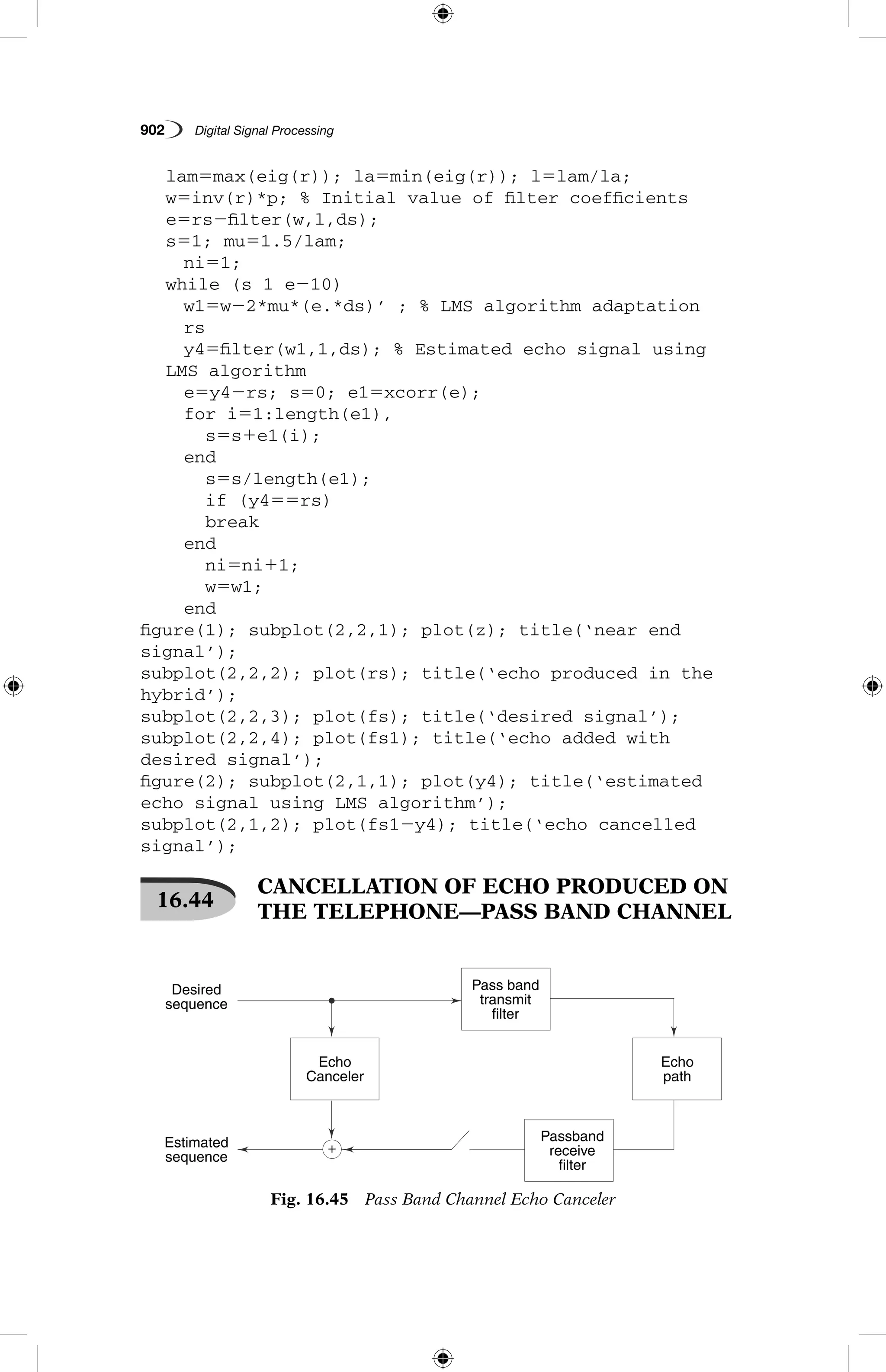
![MATLAB Programs 903
% Simulation program for passband echo cancellation
shown in Fig. 16.45 using LMS algorithm
clc; close all; clear all;
format long
fd58000; fs516000; fc58000;
f54000; t50:.01:1; %d5sin(2*pi*f*t/fd);
% Near end signal
ns5[5 2 5 2 5 5 2 2 2 5 5 2 2 2 2 2 2 5 5 2 5 2 5 5 5 5 5 5 5 5 5 5 5 5 5 5];
% Near end input signal is digitally modulated and
plotted
y5dmod(ns,fc,fd,fs,‘psk’);
subplot(2,2,1); plot(y); title(‘input signal’);
xlabel(‘Time ———’); ylabel(‘Amplitude ———’);
% Echo is generated due to mismatch of hybrid impedances
h55*randn(1,length(ns));———
rsl5filter(h,1,y);
% for i51; length(ns);
% rsl(i)5rs6(i);
% end
for i51; length(ns);
rs(i)5rs1(i);
end
subplot(2,2,2); plot(rs); title(‘noise signal’);
xlabel(‘Time ———’); ylabel(‘Amplitude ———’);
% Far end signal
fs15[5 5 2 5 2 5 2 5 2 5 2 5 2 5 5 5 5 5 5 5 5 5 2 2 2 2 2 2 2 2 2 2 2 2 2 5];
% rs5sign(rs2);
% Far end signal is digitally modulated and plotted
z15dmod(fs1,fc,fd,fs,‘psk’);
for i51:length(ns),
z(i)5z1(i);
end
subplot(2,2,3); plot(z); title(‘far-end signal’);
xlabel(‘Time ———’); ylabel(‘Amplitude ———’);
% Echo and the far end modulated signal is added in the
hybrid
q15z11rs1;
for i51; length(ns);
q(i)5q1(i);;
end
subplot(2,2,4); plot(q); title(‘received signal’);
xlabel(‘Time ———’); ylabel(‘Amplitude ———’);
q25xcorr(q);
% Auto correlation is taken for the near end signal
ar5xcorr(ns);
% cross correction is taken for the near end and far end
signal
crd5xcorr(rs,ns);](https://image.slidesharecdn.com/matlabprograms-150130053105-conversion-gate01/75/Matlab-programs-89-2048.jpg)
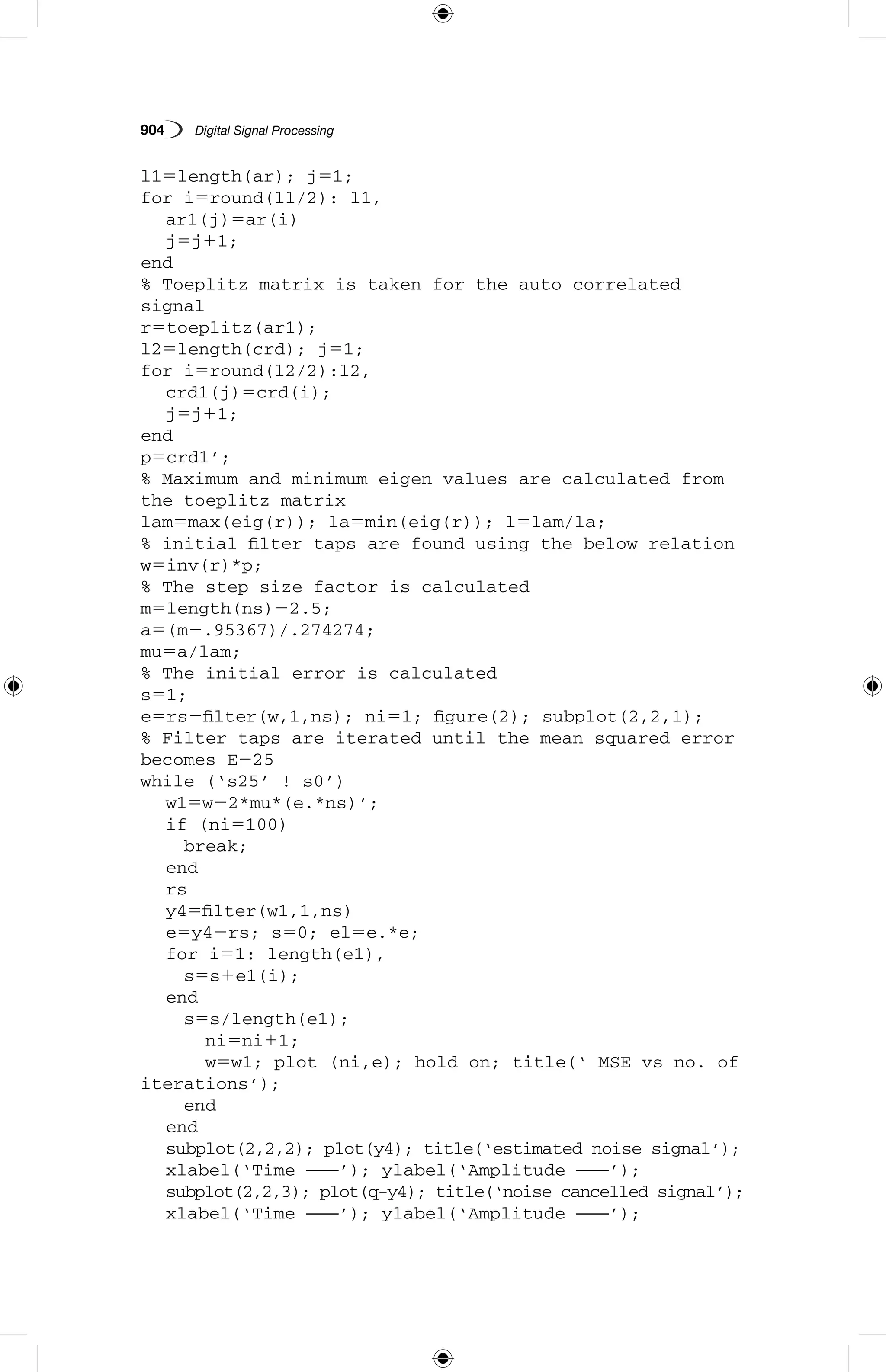
![MATLAB Programs 905
Review Questions
16.1 (a) Generate unit impulse function
(b) Generate signal x(n)5u(n) 2 u(n 2 N)
(c) Plot the sequence, x(n)5A cos ((2p f n)/fs
), where n50 to 100
fs
5100 Hz, f51 Hz, A50.5
(d) Generate x (n)5exp (25n), where n50 to 10.
16.2 Consider a system with impulse response
h n
nn
( )
( / ) ,
.
=
=
1 2 0 to 4
0, elsewhere
16.3 Consider the figure.
Fig. Q16.3
h (n)1 h (n)2
h (n)3 h (n)4
( )
y(n)
( )−
Fig. Q16.4
( ) H1 H2
H3
y (n)3
y(n)
3 (n)
H4
(a) Express the overall impulse response in terms of h1
(n), h2
(n), h3
(n), h4
(n)
(b) Determine h(n) when h1
(n)5{1/2, 1/4, 1/2}
h2
(n)5h3
(n)5(n 1 1) u(n)
h4
(n)5d(n 2 2)
(c) Determine the response of the system in part (b) if x(n)5 d(n 1 2)
1 3d(n 2 1) 2 4d(n 2 3).
16.4 Compute the overall impulse response of the system
for 0 # n # 99. The system H1
, H2
, H3
, H4
, are specified by
H1
: h1
[n]5{1, 1/2, 1/4, 1/8, 1/16, 1/32}
H2
: h2
[n]5{1, 1, 1, 1, 1}
H3
: y3
[n]5(1/4) x(n) 1 (1/2) x(n 2 1) 1 (1/4) x(n 2 2)
H4
: y[n]50.9 y(n 2 1) 2 0.81 y(n 2 2) 1 V(n) 1 V(n 2 1)
Plot h(V) for 0 # n # 99.
16.5 Consider the system with h(n)5an
u(n), 21 , a , 1. Determine the response.
x(n)5u(n 1 5) 2 u(n 2 10)](https://image.slidesharecdn.com/matlabprograms-150130053105-conversion-gate01/75/Matlab-programs-91-2048.jpg)
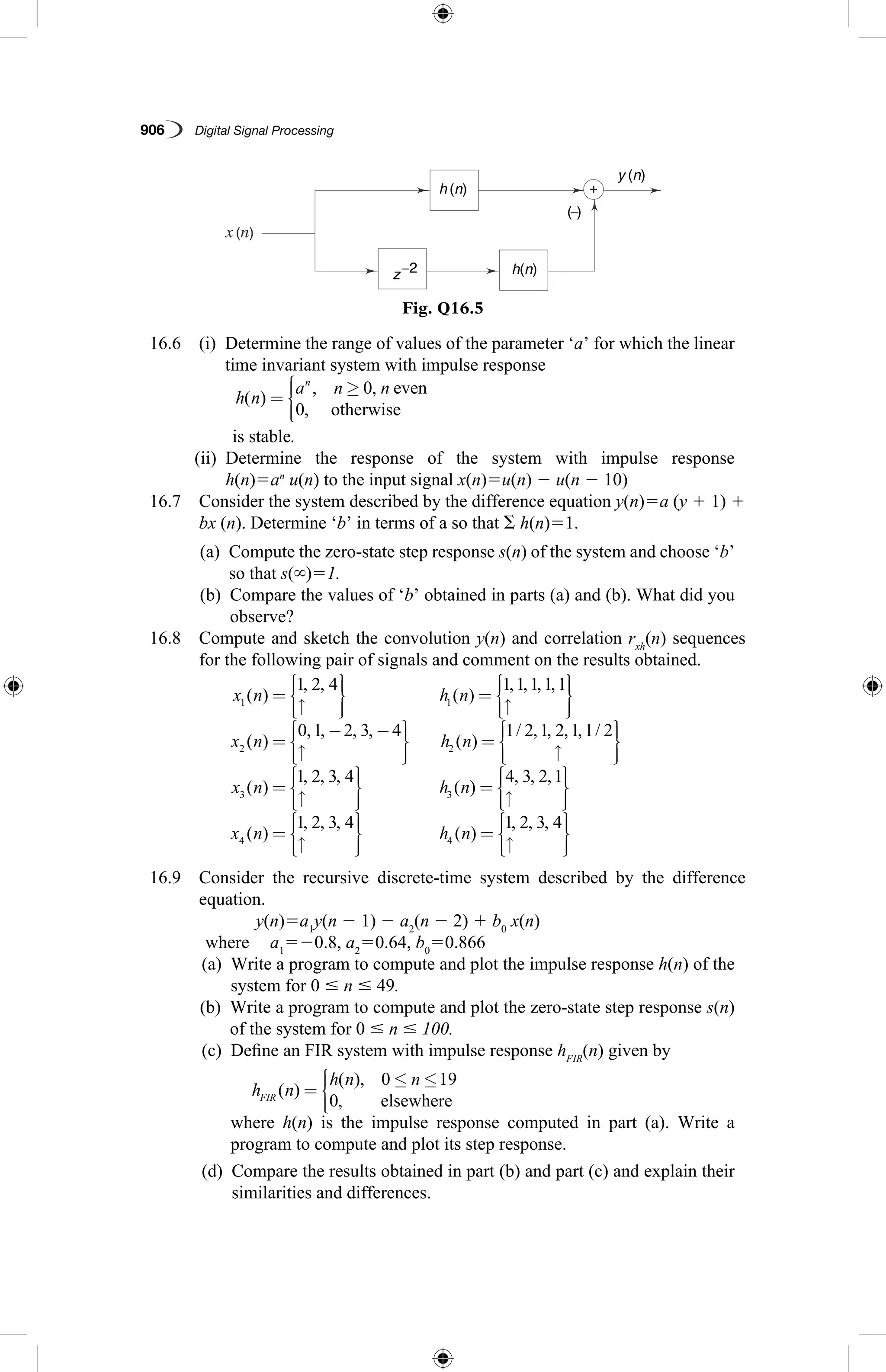
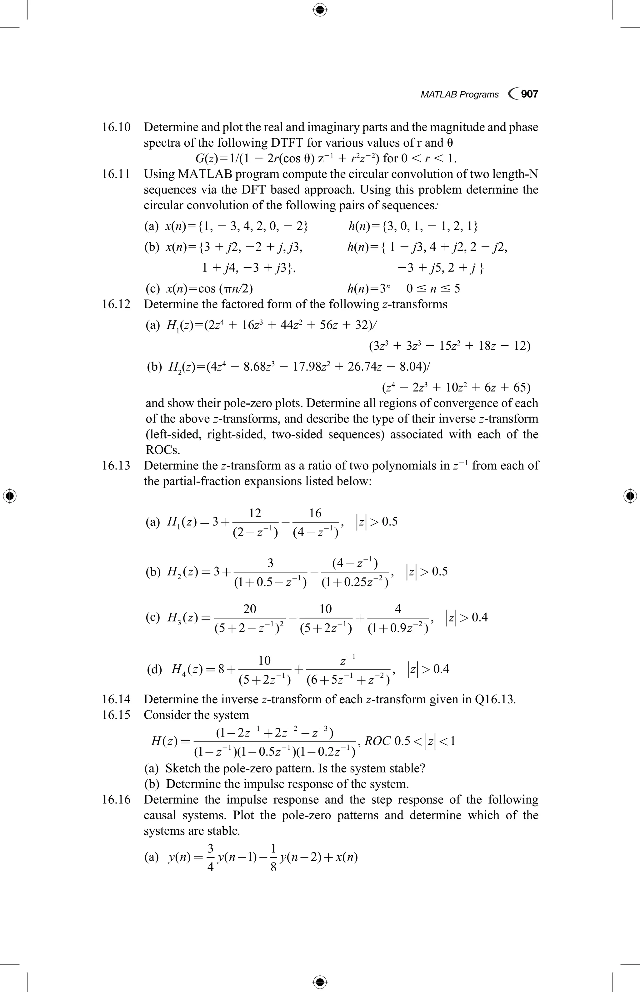
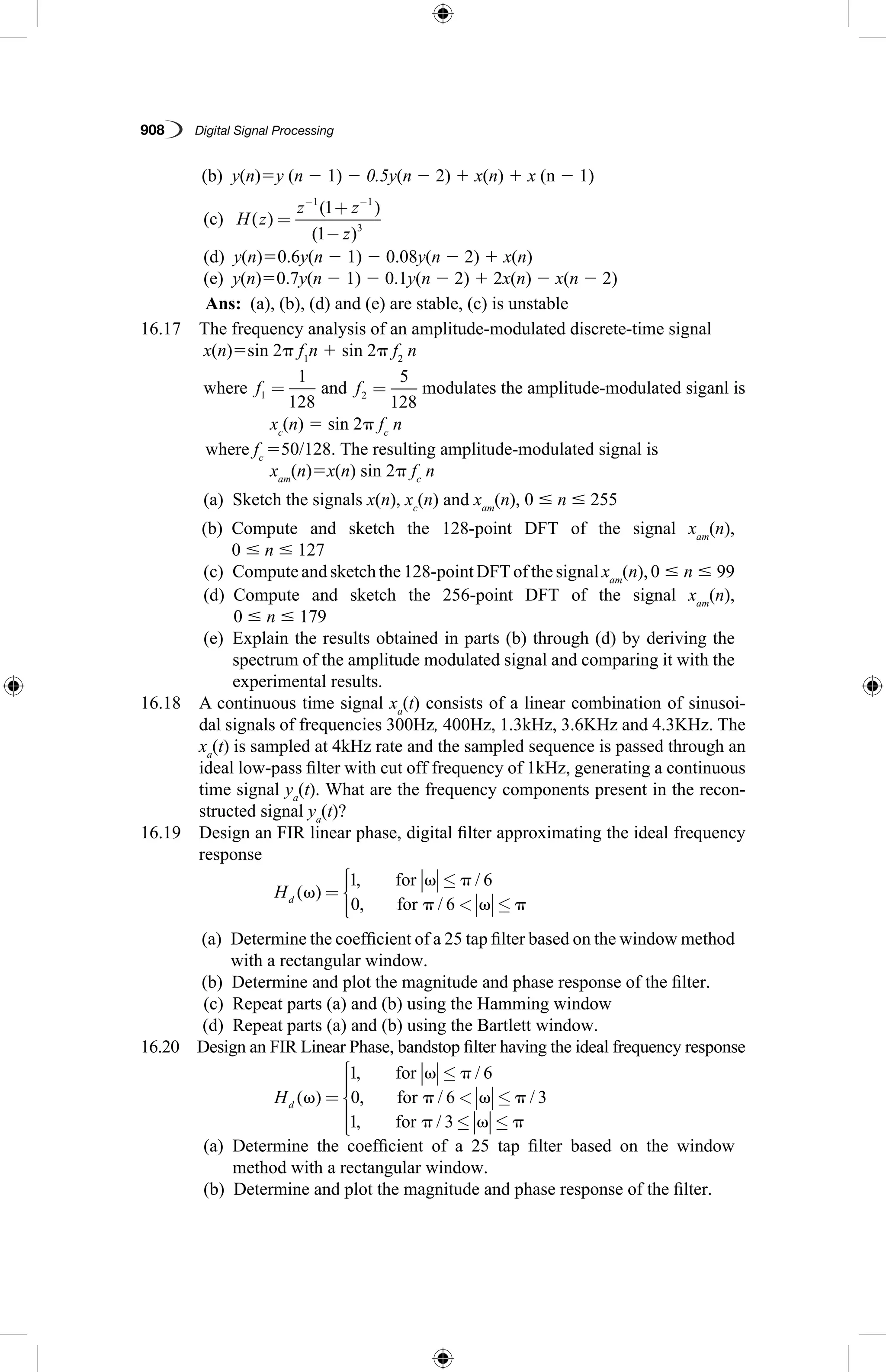

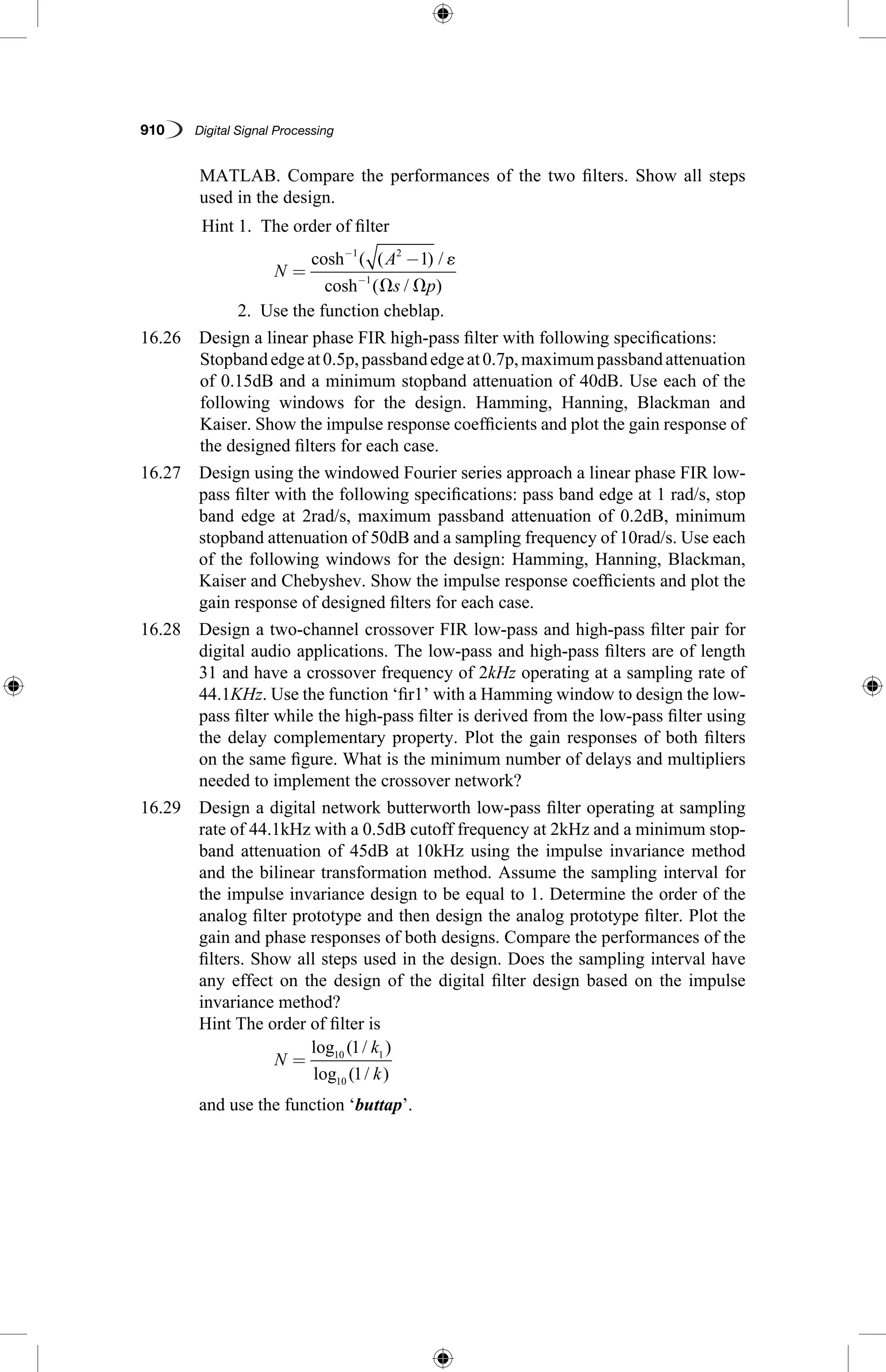


![ANPARA THERMAL POWER STATION[1] sangam.pdf](https://cdn.slidesharecdn.com/ss_thumbnails/anparathermalpowerstation1sangam-251121115219-9261cde4-thumbnail.jpg?width=640&height=640&fit=bounds)


