Downloaded 103 times
![ECE324: DIGITAL SIGNAL PROCESSING LABORATORY
Practical No.:4
Roll No: B-54 Registration No.:11205816_ Name:Shyamveer Singh
Aim: To perform DFT and IDFT of two given signals, Plot the
Magnitude and phase of same.
Mathematical Expressions Required:
1. DFT
2. IDFT
Inputs :
X(n)=[1 2 3 4 5]
X(k)=[2 4 6 8 9]
Program Codes:
1. DFT
function[y]=shyamdft(x)
m=length(x);
xk=zeros(1,m);
for k=0:m-1;
for n=0:m-1;
xk(k+1)=xk(k+1)+x(n+1)*exp((-i)*2*pi*k*n/m);
end
end
y=xk
M=sqrt(real(y).^2+imag(y).^2)
M1=abs(y)
A = atan2(imag(y),real(y))
A1=angle(y)
z=fft(x)
2. IDFT
function[y]=shyamidft(x)
m=length(x);
xk=zeros(1,m);
for k=0:m-1;
for n=0:m-1;
xk(k+1)=xk(k+1)+(1/m)*x(n+1)*exp((i)*2*pi*k*n/m)
;
end
end
y=xk
M=sqrt(real(y).^2+imag(y).^2)
M1=abs(y)
A = atan2(imag(y),real(y))
A1=angle(y)
z=ifft(x)
Outputs/ Graphs/ Plots:](https://image.slidesharecdn.com/11205816124547b-54-150415060149-conversion-gate01/85/DFT-and-IDFT-Matlab-Code-1-320.jpg)
![>> x=[1 2 3 4 5]
x=
1
2
3
4
5
>> shyamdft(x)
y=
15.0000
- 3.4410i
M=
15.0000
M1 =
15.0000
A=
0
A1 =
0
z=
15.0000
- 3.4410i
-2.5000 + 3.4410i
-2.5000 + 0.8123i
-2.5000 - 0.8123i
-2.5000
2.1991
2.8274
-2.8274
-2.1991
2.1991
2.8274
-2.8274
-2.1991
4.2533
2.6287
2.6287
4.2533
4.2533
2.6287
2.6287
4.2533
-2.5000 + 3.4410i
-2.5000 + 0.8123i
-2.5000 - 0.8123i
-2.5000
Comparison with inbuilt functions: A= angle or phase, M=magnitude compare with
inbuilt commands abs, angle.
Y is output Compare with Z inbuilt command.
Outputs/ Graphs/ Plots:
2. IDFT
x=[2 4 6 8 9]
x=
2
4](https://image.slidesharecdn.com/11205816124547b-54-150415060149-conversion-gate01/85/DFT-and-IDFT-Matlab-Code-2-320.jpg)
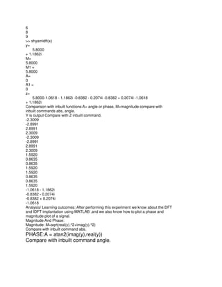

This document describes an experiment to perform the discrete Fourier transform (DFT) and inverse discrete Fourier transform (IDFT) on two input signals using MATLAB. The experiment calculates the magnitude and phase of the DFT and IDFT outputs and compares the results to the MATLAB FFT and IFFT functions. The student learns how to implement the DFT and IDFT and plot the magnitude and phase of signals.


![Multiband Transceivers - [Chapter 3] Basic Concept of Comm. Systems](https://cdn.slidesharecdn.com/ss_thumbnails/ch3-150613070933-lva1-app6892-thumbnail.jpg?width=640&height=640&fit=bounds)