digital signal-processing-lab-manual

JAYALAKHSMI
INSTITUTE OF TECHNOLOGY
NH -7 Thoppur, Dharmapuri District
Department of Electronics and Communication Engineering
080290034 DIGITAL SIGNAL PROCESSING
LABORATORY MANUAL
ECE V SEMESTER

080290034 Digital signal processing lab ECE V Sem
EXTRACT OF UNIVERSITY SYLLABUS
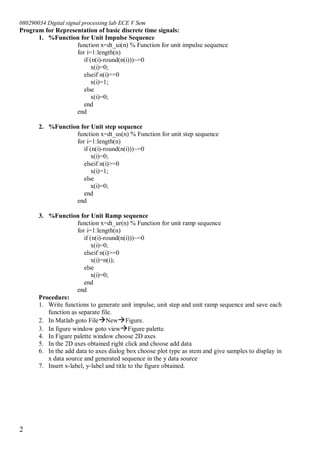
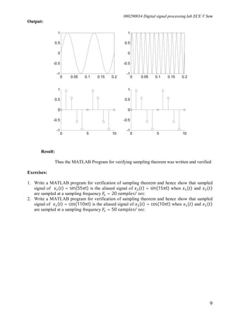
080290034 DIGITAL SIGNAL PROCESSING LAB
USING TMS320C5X
1. Generation of Signals
2. Linear Convolution
3. Implementation of a FIR filter
4. Implementation of an IIR filter
5. Calculation of FFT
USING MATLAB
1. Generation of Discrete time Signals
2. Verification of Sampling Theorem
3. FFT and IFFT
4. Time & Frequency response of LTI systems
5. Linear and Circular Convolution through FFT
6. Design of FIR filters (window design)
7. Design of IIR filters (Butterworth &Chebychev)

LIST OF EXPERIMENTS
S. No. Experiment Name Page No.
USING MATLAB
1. (a) Representation of basic discrete time signals 1
(b) Generation of periodic Signals 4
2. Verification of sampling theorem 7
3. Calculation of FFT and IFFT of a sequence 10
4. Time & Frequency response of LTI systems 13
5. Linear and Circular Convolution through FFT 16
6. Design of FIR filter using windows 19
7. Design of IIR filters from Chebychev analog filters 24
8. Design of IIR filters from Butterworth analog filters 28
USING TMS320C5416
9. Linear Convolution 33
10. Circular Convolution 35
11. Calculation of FFT 37
12. Generation of Signals 43
13. Implementation of a IIR filter 46
14. Implementation of a FIR filter 51

1
Exp No: 1(a) Date : _ _/_ _/_ _
REPRESENTATION OF BASIC DISCRETE TIME SIGNALS
Aim:
To write a MATLAB program to generate various input Waveforms.
Tools and Software Required:
HARDWARE: IBM PC (Or) Compatible PC
SOFTWARE: MATLAB 6.5 (Or) High version
Theory:
Discrete time signal
Functional
representation
Unit impulse sequence [ ] =
1, = 0
0,
Unit step sequence [ ] =
1, ≥ 0
0,
Unit ramp sequence [ ] =
1, ≥ 0
0,
Exponential sequence [ ] =
sinusoidal sequence [ ] = sin ( )
Algorithm:
Step 1: Input no. of samples to display
Step 2: Generate the sequence
Step 3: Plot the sequence
Flow chart:
Start
Input no. of samples to
display
Generate the sequence
Plot the sequence for given
samples
Stop

2
Program for Representation of basic discrete time signals:
1. %Function for Unit Impulse Sequence
function x=dt_ui(n) % Function for unit impulse sequence
for i=1:length(n)
if (n(i)-round(n(i)))~=0
x(i)=0;
elseif n(i)==0
x(i)=1;
else
x(i)=0;
end
end
2. %Function for Unit step sequence
function x=dt_us(n) % Function for unit step sequence
for i=1:length(n)
x(i)=0;
elseif n(i)>=0
x(i)=1;
else
x(i)=0;
end
end
3. %Function for Unit Ramp sequence
function x=dt_ur(n) % Function for unit ramp sequence
for i=1:length(n)
x(i)=0;
elseif n(i)>=0
x(i)=n(i);
else
x(i)=0;
end
end
Procedure:
1. Write functions to generate unit impulse, unit step and unit ramp sequence and save each
function as separate file.
2. In Matlab goto FileNewFigure.
3. In figure window goto viewFigure palette.
4. In Figure palette window choose 2D axes
5. In the 2D axes obtained right click and choose add data
6. In the add data to axes dialog box choose plot type as stem and give samples to display in
x data source and generated sequence in the y data source
7. Insert x-label, y-label and title to the figure obtained.

3
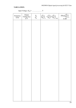
Output:
Result:
Thus the MATLAB Program for representation of signals was written and verified.
Exercises:
1. Write a MATLAB program to represent unit step sequence ( [ ]) and hence sketch the
following sequence [ ] = [ ] − [ − ] + [ − ].
2. Write a MATLAB program to represent unit sample sequence ( [ ]) and unit step sequence
( [ ]) and hence sketch the following sequence
[ ] = [ + ] − [ ] + [ + ] − [ − ].
3. Write a MATLAB program to represent unit step sequence ( [ ]) and unit ramp sequence
( [ ]) and hence sketch the following sequence [ ] = [ + ] − [ ] − [ − ].
4. Write a MATLAB program to represent unit step sequence ( [ ]) and exponential sequence
and hence sketch the following sequence [ ] = . [ + ] + [ ].
5. Write a MATLAB program to represent sinusoidal sequence and exponential sequence and
hence sketch the following sequence [ ] = ( . ) [ ( / ) + ( / )].
6. Write a MATLAB program to represent unit step sequence ( [ ]) and exponential sequence
and hence sketch the following sequence [ ] = (− . ) [ ].
-10 -5 0 5 10
0
0.5
1
Unit Impulse Sequence
n
amp.
-10 -5 0 5 10
0
0.5
1
Unit Step Sequence
n
amp.-10 -5 0 5 10
0
5
10
Unit Ramp Sequence
n
amp.
-10 -5 0 5 10
0
5
10
Exponential (Growing)
n
amp.
-10 -5 0 5 10
0
5
10
Exponential (Decaying)
n
amp.
-10 -5 0 5 10
-1
0
1
Sinusoidal
n
amp.

4
Exp No: 1(b) Date : _ _/_ _/_ _
GENERATION OF PERIODIC SIGNALS
Aim:
To write a MATLAB program to generate various periodic signals.
HARDWARE: IBM PC (Or) Compatible PC
SOFTWARE: MATLAB 6.5 (Or) High version
Theory:
Periodic sinusoidal sequence can be generated using the following iterative function
sin( ) = sin( ( − 1)) ∗ cos( ) + cos( ( − 1)) ∗ sin( )
cos( ) = cos( ( − 1)) ∗ cos( ) − sin( ( − 1)) ∗ sin ( )
where, = , → period of the sequence (a rational number)
Other periodic signals ( ) can be generated using trigonometric Fourier series given
by
( ) = [0] + ( [ ] cos( ) + [ ] sin( ))
where, = , → period of the signal and
[0] = ∫ ( )
[ ] = ∫ ( )cos ( ) ,
[ ] = ∫ ( )sin ( )
[0], [ ] [ ] are trigonometric Fourier series coefficients
Algorithm:
Step 1: Input period for the periodic signal
Step 2: Generate the sinusoidal sequence for given period
Step 3: Determine Fourier series coefficients for given periodic signal
Step 4: Generate periodic signal using trigonometric Fourier series

5
Flow chart:
Program for Generation of periodic signals:
1. %Function for sinusoidal sequence generation
function [sint,cost] = swg(n,N)
sinp = 0;
cosp = 1;
sini = sin(2*pi/N);
cosi = cos(2*pi/N);
sint = [sinp sini zeros(1,n-1)];
cost = [cosp cosi zeros(1,n-1)];
for i=2:n+1
sint(i) = sinp*cosi + cosp*sini;
cost(i) = cosp*cosi - sinp*sini;
sinp = sint(i);
cosp = cost(i);
end
2. %Program for square wave generation
clc;
clear all;
close all;
n = 400;
ps = zeros(1,n+1);
for i=1:5
[st,ct]=swg(n,200/(2*i-1));
ps = ps+2*st/(pi*(2*i-1));
end
ps = ps + 0.5;
plot((0:n)/200,ps)
Start
Input Period of the periodic
signal
Generate the sinusoidal
sequence for given period
Generate and plot the
periodic signal
Stop

6
Output:
Result:
Thus the MATLAB Program for generation of periodic signals was written and
verified.
Exercises:
1. Write a MATLAB program to generate triangular waveform given by
2. Write a MATLAB program to generate sawtooth waveform given by
-5 -4 -3 -2 -1 0 1 2 3 4 5
0
0.5
1
x(t)-triangular pulse, |t|,-1<t<1
|c[n]|
-5 -4 -3 -2 -1 0 1 2 3 4 5
-1
0
1
x(t)=t, -1<t<1
|c[n]|

7
Exp No: 2 Date : _ _/_ _/_ _
VERIFICATION OF SAMPLING THEOREM
Aim:
To write the program for verification of sampling theorem using MATLAB.
HARDWARE: IBM PC (OR) Compatible PC
SOFTWARE: MATLAB 6.5 (OR) High version
Theory:
Discrete-time signal [ ] is obtained by taking samples of analog signal ( ) every
seconds, which is described by the relation
[ ] = ( ), −∞ < < ∞
The timing interval between successive samples is called the sampling period or
sampling interval and its reciprocal = is called the sampling rate or the sampling
frequency.
Let be − < < the frequencies = + , −∞ < < ∞, are
indistinguishable from after sampling and hence they are aliases of .
Hence to avoid aliasing is selected so that > 2 , where is the largest
frequency component in the analog signal ( ).
Algorithm:
1. Choose fundamental frequency (F0) for a sinusoidal signal and sampling rate (Fs)
according to Nyquist theorem.
2. Choose another sinusoidal signal of frequency F=F0+kFs, where k is an non-zero
integer.
3. Display both sinusoidal signal for some time duration 0 to T.
4. Display the sampled sinusoidal signals for above time duration, sampled at the rate
Fs.

8
Flow chart:
Program for Sampling and aliasing:
clc;
clear all;
close all;
% continous time signal
f0 = 10; % fundmental frequency
fs = 50; % Sampling frequency
f = 60; % Alias frequency f = f0+ k*fs
t=0:1/(20*f):2/f0; % time scale
% program to generate sinusoidal signal of frequency f0
csf0 = sin(2*pi*f0*t);
% program to generate sinusoidal signal of frequency f = f0 + k*fs
csf = sin(2*pi*f*t);
% discrete time signal
n = 0:10; % time scale
% program to generate sinusoidal signal of freq. f0 sampled at the rate fs
ssf0 = sin(2*pi*f0*n/fs);
% program to generate sinusoidal signal of freq. f sampled at the rate fs
ssf = sin(2*pi*f*n/fs);
% program to plot the signals
subplot(2,2,1)
plot(t,csf0);
subplot(2,2,2)
plot(t,csf);
subplot(2,2,3)
stem(n,ssf0);
subplot(2,2,4)
stem(n,ssf);
Start
Input fundamental frequency F0 of sinusoidal signal,
sampling rate Fs and another sinusoidal signal of
frequency F=F0+kFs
Display both sinusoidal signal for time duration 0 to T
Display the sampled sinusoidal signals for the above
time duration, sampled at the rate Fs
Stop

9
Output:
Result:
Thus the MATLAB Program for verifying sampling theorem was written and verified
Exercises:
1. Write a MATLAB program for verification of sampling theorem and hence show that sampled
signal of ( ) = sin(55πt) is the aliased signal of ( ) = sin(15πt) when ( ) and ( )
are sampled at a sampling frequency = 20 / .
2. Write a MATLAB program for verification of sampling theorem and hence show that sampled
signal of ( ) = cos(110πt) is the aliased signal of ( ) = cos(10πt) when ( ) and ( )
are sampled at a sampling frequency = 50 / .
0 0.05 0.1 0.15 0.2
-1
-0.5
0
0.5
1
0 0.05 0.1 0.15 0.2
-1
-0.5
0
0.5
1
0 5 10
-1
-0.5
0
0.5
1
0 5 10
-1
-0.5
0
0.5
1

10
Exp No: 3 Date : _ _/_ _/_ _
CALCULATION OF FFT AND IFFT OF A SEQUENCE
Aim:
To write a MATLAB program for computing FFT of a Signal
Theory:
N-point DFT of a discrete sequence [ ] is given by
[ ] = [ ] = [ ] , ℎ = 0,1, … − 1 =
N-point IDFT is given by
[ ] = [ ] =
1
[ ]
∗
, ℎ = 0,1, … − 1
Algorithm:
1. Get the input sequence.
2. Compute the DFT and IDFT using FFT and IFFT fuction
3. Plot the input sequence, real part, imaginary part, magnitude spectrum and phase
spectrum of the DFT obtained and IFFT sequence obtained

11
Flow chart:
Program for calculation of FFT and IFFT:
clc;
clear all;
close all;
x = [1 2 1 2 1 2 1 2]; % enter the input sequence
n=0:length(x)-1;
X = fft(x); % DFT of the sequence
y = ifft(X); % IDFT of the sequence
% Program to plot the sequence
subplot(3,2,1)
stem(n,x);
subplot(3,2,2)
stem(n,real(X));
subplot(3,2,3)
stem(n,imag(X));
subplot(3,2,4)
stem(n,abs(X));
subplot(3,2,5)
stem(n,angle(X));
subplot(3,2,6)
stem(n,y);
Start
Input a sequence
Compute DFT and IDFT using FFT and IFFT
Plot the magnitude spectrum and Phase Spectrum for
the DFT of the given input sequence
Stop

12
Output:
Result:
Thus the MATLAB Program for computing of DFT using FFT was Written and
verified.
Exercises:
1. Write a MATLAB program for computation of FFT and IFFT and hence verify the symmetry
property, DFT of the real and even sequence is real and even for the sequence [ ] =
{1,1,1,0,0,0,1,1}.
2. Write a MATLAB program for computation of FFT and IFFT and hence verify the symmetry
property, DFT of the real and odd sequence is purely imaginary and odd for the sequence
[ ] = {0,1,1,0,0,0, −1, −1}.
0 2 4 6 8
0
1
2
0 2 4 6 8
-10
0
10
20
0 2 4 6 8
-1
0
1
0 2 4 6 8
0
5
10
15
0 2 4 6 8
0
2
4
0 2 4 6 8
0
1
2

13
Exp No: 4 Date : _ _/_ _/_ _
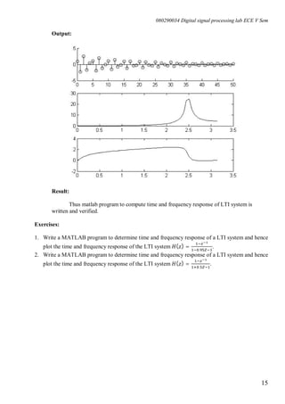
TIME & FREQUENCY RESPONSE OF LTI SYSTEMS
Aim:
To write a MATLAB program to compute time and frequency response of LTI
system.
Theory:
Time domain response ℎ[ ] of LTI system ( ) is given by
( ) =
( )
( )
Frequency domain response ( ) of LTI system ( ) is given by
=
( )
( )
Algorithm:
1. Get the Numerator and denominator coefficients of a LTI system ( ).
2. Compute impulse response h[n] of the LTI system
3. Compute frequency response ( ) of the LTI system ( )
4. Plot the impulse response and magnitude and phase of frequency response

14
Flow chart:
Program for time and frequency response of LTI system:
clc;
clear all;
close all;
num = [1 -0.8]; den = [1 1.5 0.9]; % Nr. & Dr. of LTI system H(Z)
N = 50;
h = impz(num,den,N+1); % Time response or impulse response h[n]
[H w] = freqz(num,den,0:pi/50:pi); % Frequency response H(e^(jw))
% Program to plot the responce
subplot(3,1,1)
stem(0:N,h);
subplot(3,1,2)
stem(w,abs(H));
subplot(3,1,3)
stem(w,angle(H));
Start
Input the Numerator and denominator coefficients of a
LTI system ( )
Compute impulse response and frequency response
Plot the impulse response and magnitude and phase of
frequency response
Stop

15
Output:
Result:
Thus matlab program to compute time and frequency response of LTI system is
written and verified.
Exercises:
1. Write a MATLAB program to determine time and frequency response of a LTI system and hence
plot the time and frequency response of the LTI system ( ) =
.
.
2. Write a MATLAB program to determine time and frequency response of a LTI system and hence
plot the time and frequency response of the LTI system ( ) =
.
.

16
Exp No: 5 Date : _ _/_ _/_ _
LINEAR AND CIRCULAR CONVOLUTION THROUGH FFT
Aim:
To write a program for linear convolution and circular convolution using MATLAB.
Theory:
Linear convolution [ ] for the sequence [ ] and ℎ[ ] is given by
[ ] = ∑ [ ]ℎ[ − ] (1)
N-point Circular convolution [ ] for the sequence [ ] and ℎ[ ] is given by
[ ] = ∑ [ ]ℎ[( − ) ] , ℎ = 0,1, … − 1 (2)
Using circular convolution property of DFT circular convolution [ ] is obtained by
[ ] = [ ( [ ] ) (ℎ[ ] )] (3)
Linear convolution [ ] for the sequence [ ] of length m and ℎ[ ] of length l is obtained by
computing N-point circular convolution between x[n] and h[n], where N = m+l-1.
Algorithm:
1. Enter the value for the sequence [ ] and ℎ[ ].
2. Compute the linear convolution using the equation (1)
3. Compute the circular convolution using the equation (2)
4. Verify the result through circular convolution property of DFT
5. Display the input sequences, output linear and circular convolution sequences.
Flow chart:
Start
Input a sequence x and h
Compute Linear convolution and circular convolution
using equation (1) & (2)
Compute Linear convolution and circular convolution
using circular convolution property of DFT
Stop

17
Program for computation of linear and circular convolution:
clc;
clear all;
close all;
x = [1 2 3 4]; % enter the sequence x[n]
h = [1 2 1 2]; % enter the sequence h[n]
ylc=conv(x,h); % compute linear conolution
m=length(x);
n=length(h);
L=m+n-1; % no. of samples in linear convolution
% program to compute Circular convolution
N=max(m,n); % no. of samples in circular convolution
if m<n
x=[x zeros(1,N-m)];
else
h=[h zeros(1,N-n)];
end
for k=0:N-1
sum=0;
for j=0:N-1
sum=sum+x(j+1)*h(mod(k-j,N)+1);
end
ycc(k+1)=sum;
end
% program to compute linear and circular convolution through FFT
ycc_fft = ifft(fft(x).*fft(h)); % Circular convolution
x = [x zeros(1,L-N)];
h = [h zeros(1,L-N)];
ylc_fft = ifft(fft(x).*fft(h)); % Linear convolution
% program to plot the sequence
subplot(4,1,1)
stem(0:L-1,x);
subplot(4,1,2)
stem(0:L-1,h);
subplot(4,1,3)
stem(0:N-1,ycc_fft);
subplot(4,1,4)
stem(0:L-1,ylc_fft);

18
Output:
Result:
Thus the MATLAB Program for Linear and Circular convolution written and verified.
Exercises:
1. Write a MATLAB program for computation of Linear Convolution through FFT and hence
compute linear convolution between the sequence [ ] = {−3,2,4} and [ ] = {2, −4,0,1}
through FFT.
2. Write a MATLAB program for computation of Circular Convolution through FFT and hence
compute circular convolution between the sequence [ ] = {−2,1, −3,4} and [ ] = {1,2, −3,2}
through FFT.
0 1 2 3 4 5 6
0
2
4
0 1 2 3 4 5 6
0
1
2
0 0.5 1 1.5 2 2.5 3
0
10
20
0 1 2 3 4 5 6
0
10
20

19
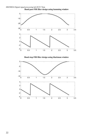
Exp No: 6 Date : _ _/_ _/_ _
Design of FIR filter using windows
Aim:
To write a MATLAB program to design a FIR filter by using Windowing techniques.
Theory:
Impulse response of a FIR filter using windowing technique is given by,
ℎ[ ] = ℎ [ ] [ ], 0 ≤ ≤ − 1
where, ℎ [ ]-desired impulse response, [ ]-window function and -is FIR filter
length
and ℎ[ ] must satisfy the linear phase condition ℎ[ ] = ℎ[ − 1 − ]
Desired frequency response ( ) and impulse response ℎ [ ] for various filter
Filter Ideal frequency response Ideal impulse response
Low pass filter ( ) =
1, | | ≤
0, < | | <
ℎ [ ] =
, = 0
sin ( )
, n ≠ 0
High Pass filter ( ) =
1, ≤ | | ≤
0, | | <
ℎ [ ] =
1 − , = 0
−
sin ( )
, n ≠ 0
Band pass filter ( ) =
1, ≤ | | ≤
0, < | | < | | <
ℎ [ ] =
−
, = 0
sin( ) − sin ( )
, n ≠ 0
Band stop or
band reject filter
( ) =
1, ≤ | | ≤ | | ≤
0, < | | <
ℎ [ ] =
1 −
−
, = 0
sin( ) − sin ( )
, n ≠ 0
where, -cut-off frequency of low pass and high pass filter,
, - lower and upper cut-off frequencies of band pass and band stop filter
Window functions, [ ] 0 ≤ ≤ − 1, where, -is FIR filter length
Rectangular window [ ] = 1
Hanning window [ ] =
1
2
1 −
2
− 1
Hamming Window [ ] = 0.54 − 0.46
2
− 1
Blackman window [ ] = 0.42 − 0.5
2
− 1
+ 0.08
4
− 1

20
Algorithm:
1. Get the order of the filter and normalized cut-off frequency and filter type
2. Get the coefficients of the filter by using window functions
3. Calculate frequency response
4. Plot the frequency response
Flow chart:
Program for Design and analysis of FIR filter using windows:
clc;
clear all;
close all;
% low pass FIR filter design using rectangular window
h_lp=fir1(10,0.25,rectwin(11));
[H_lp w]=freqz(h_lp);
figure(1)
subplot(2,1,1)
plot(w,20*log10(abs(H_lp)));
subplot(2,1,2)
plot(w,angle(H_lp));
% high pass FIR filter design using hanning window
h_hp=fir1(10,0.5,'high',hann(11));
[H_hp w]=freqz(h_hp);
figure(2)
subplot(2,1,1)
plot(w,20*log10(abs(H_hp)));
subplot(2,1,2)
plot(w,angle(H_hp));
% band pass FIR filter design using hamming window
h_bp=fir1(10,[0.25 0.75],hamming(11));
[H_bp w]=freqz(h_bp);
figure(3)
subplot(2,1,1)
plot(w,20*log10(abs(H_bp)));
subplot(2,1,2)
Start
Input a order of the filter and normalized cut-off
frequency and filter type
Compute filter coefficients using various window
techniques
Compute and plot the frequency response of the filter
Stop

21
plot(w,angle(H_bp));
% band stop FIR filter design using blackman window
h_bs=fir1(10,[0.25 0.75],'stop',blackman(11));
[H_bs w]=freqz(h_bs);
figure(4)
subplot(2,1,1)
plot(w,20*log10(abs(H_bs)));
subplot(2,1,2)
plot(w,angle(H_bs));
Output :
Low pass FIR filter design using rectangular window
High pass FIR filter design using hanning window
0 0.5 1 1.5 2 2.5 3 3.5
-80
-60
-40
-20
0
0 0.5 1 1.5 2 2.5 3 3.5
-4
-2
0
2
4
0 0.5 1 1.5 2 2.5 3 3.5
-100
-50
0
50
0 0.5 1 1.5 2 2.5 3 3.5
-4
-2
0
2
4

22
Band pass FIR filter design using hamming window
Band stop FIR filter design using blackman window
0 0.5 1 1.5 2 2.5 3 3.5
-30
-20
-10
0
0 0.5 1 1.5 2 2.5 3 3.5
-4
-2
0
2
4
0 0.5 1 1.5 2 2.5 3 3.5
-15
-10
-5
0
0 0.5 1 1.5 2 2.5 3 3.5
-4
-2
0
2
4

23
Result:
Thus the MATLAB Program for FIR filter using windowing techniques is designed
and verified.
Exercises:
1. Write a MATLAB program to design digital high pass Linear phase FIR filter with cut-off
frequency = . Using rectangular window of length 11.
2. Write a MATLAB program to design digital low pass Linear phase FIR filter with cut-off
frequency = 0.5 . Using Hamming window of length 9.
3. Write a MATLAB program to design digital band pass Linear phase FIR filter with cut-off
frequencies = 0.25 and = 0.75 . Using Hanning window of length 11.
4. Write a MATLAB program to design digital band stop Linear phase FIR filter with cut-off
frequencies = and = . Using Blackman window of length 9.

24
Exp No: 7 Date : _ _/_ _/_ _
Design of IIR filters from Chebychev analog filters
Aim:
To write a program to design a chebyshev low pass filter
1.Impulse invariant method
2.Bilinear Transform using MATLAB.
Theory:
Type I Chebyshev filters are all-pole filters that exhibit equiripple behavior in the
passband and a monotonic characteristics in the stopband.
The magnitude squared of the frequency response is given as,
| (Ω)| =
1
1 + Ω Ω⁄
Where, ( ) is the th-order Chebyshev polynomial
Order of the filter is given by,
=
ℎ ( ⁄ )
ℎ (Ω Ω )⁄
Where, = − 1 and -is the stop band ripple
=
( )
− 1 and -is the pass band ripple
Ω -is the stop band edge frequency
Ω -is the pass band edge frequency
Poles of the type I Chebyshev filter lie on the ellipse at the coordinates ( , ) given
as,
= cos = 0,1, … , − 1
= sin , = 0,1, … , − 1
Where, = +
( )
is the angular positions of the poles
= Ω is the semi major axis of the ellipse
= Ω is the semi minor axis of the ellipse and =
√
⁄
Hence, analog system transfer function of type I chebyshev filter is given by,
( ) =
1
∏ ( − )
Where, = + are poles of the filter.
Impulse invariance – used to determine system transfer function of digital IIR filter
( ) from analog system transfer function using the relation
( ) = ( )|
∑ ∑
and digital frequency, = Ω , where, Ω - is analog frequency and - is sampling
period.
Bilinear transformation – used to determine system transfer function of digital IIR
filter ( ) from analog system transfer function using the relation
( ) = ( )|

25
and digital frequency, = 2 , where, Ω - is analog frequency and - is
sampling period.
algorithm:
1. Get the passband and stopband edge frequencies in rad/sec and ripples in dB
2. compute the order of the filter
3. compute the analog system transfer function
4. compute digital system transfer function of the IIR filter from analog transfer
function
5. compute and plot the frequency response of the IIR filter
Flow Chart:
Program for design of Chebyshev analog and digital filter:
clc;
clear all;
close all;
% input specification of the filter
T=1; %sampling period
wp=0.2*pi; %pass band edge frequency in radians/sample
ws=0.5*pi; %stop band edge frequency in radians/sample
rp=0.707; %passband ripple
rs=0.1; %stopband ripple
Rp=-20*log10(rp); %passband ripple in dB
Rs=-20*log10(rs); %stopband ripple in dB
%impulse invariance
Wpi=wp/T; %pass band edge frequency in radians/sec
Wsi=ws/T; %stop band edge frequency in radians/sec
[Ni wn]=cheb1ord(Wpi,Wsi,Rp,Rs,'s'); %order of type I Chebyshev
Start
Input passband and stopband edge frequencies in
rad/sec and ripples in dB
Compute order of the filter and analog system transfer
function
Compute digital system transfer function and plot the
frequency response of the IIR filter
Stop

26
[bi ai]=cheby1(Ni,rp,wn,'s'); %analog transfer function of type I Chebyshev
[Bi Ai]=impinvar(bi,ai,1/T); %digital transfer function using impulse invariance
[Hi w]=freqz(Bi,Ai); %frequency response
figure(1);
subplot(2,1,1)
plot(w,20*log10(abs(Hi)));
subplot(2,1,2)
plot(w,angle(Hi));
%Bilinear transformantion
Wpb=(2/T)*tan(wp/2); %pass band edge frequency in radians/sec
Wsb=(2/T)*tan(ws/2); %stop band edge frequency in radians/sec
[Nb wn]=cheb1ord(Wpb,Wsb,Rp,Rs,'s'); %order of type I Chebyshev
[bb ab]=cheby1(Nb,rp,wn,'s'); %analog transfer function of type I Chebyshev
[Bb Ab]=bilinear(bb,ab,1/T); %digital transfer function using impulse invariance
[Hb w]=freqz(Bb,Ab); %frequency response
figure(2);
subplot(2,1,1)
plot(w,20*log10(abs(Hb)));
subplot(2,1,2)
plot(w,angle(Hb));
Output:
Impulse invariance method:
0 0.5 1 1.5 2 2.5 3 3.5
-20
-15
-10
-5
0
0 0.5 1 1.5 2 2.5 3 3.5
-4
-3
-2
-1
0

27
Bilinear Transformation method:
Result:
Thus the MATLAB Program for a chebyshev low pass filter is designed and verified.
Exercises:
1. Write a MATLAB program to design Chebyshev digital filter with the specifications 1 dB ripple
in the pass band 0 ≤ ≤ 0.2 , 15 dB ripple in the stop band 0.5 ≤ ≤ , using impulse
invariance method.
2. Write a MATLAB program to design Chebyshev digital filter to meet the constraints
0.707 ≤ ≤ 1, 0 ≤ ≤ 0.2
≤ 0.1, 0.5 ≤ ≤
by using bilinear transformation and assume sampling
period T = 1 sec.
0 0.5 1 1.5 2 2.5 3 3.5
-150
-100
-50
0
0 0.5 1 1.5 2 2.5 3 3.5
-4
-3
-2
-1
0

28
Exp No: 8 Date : _ _/_ _/_ _
Design of IIR filters from Butterworth analog filters
Aim:
To write a program for Butterworth low pass filter by
i) Impulse invariant method
ii) Bilinear Transform using MATLAB.
Theory:
Butterworth filters are all-pole filters and monotonic in both the passband and
stopband.
The magnitude squared of the frequency response is given as,
| (Ω)| =
1
1 + (Ω Ω⁄ )
Where, Ω is the 3-dB cut-off frequency in rad/sec
Order of the filter is given by,
=
( ⁄ )
(Ω Ω )⁄
Where, = − 1 and -is the stop band ripple
=
( )
− 1 and -is the pass band ripple
Ω -is the stop band edge frequency
Ω -is the pass band edge frequency
Poles of the butterworth filter lie on the circle of radius Ω at the coordinates ( , )
given as,
= Ω cos = 0,1, … , − 1
= Ω sin , = 0,1, … , − 1
Where, = +
( )
is the angular positions of the poles
Hence, analog system transfer function of butterworth filter is given by,
( ) =
1
∏ ( − )
Where, = + are poles of the filter.
Impulse invariance – used to determine system transfer function of digital IIR filter
( ) from analog system transfer function using the relation
( ) = ( )|
∑ ∑
and digital frequency, = Ω , where, Ω - is analog frequency and - is sampling
period.
Bilinear transformation – used to determine system transfer function of digital IIR
filter ( ) from analog system transfer function using the relation
( ) = ( )|
and digital frequency, = 2 , where, Ω - is analog frequency and - is
sampling period.

29
Algorithm:
1. Get the passband and stopband edge frequencies in rad/sec and ripples in dB
2. compute the order of the filter
3. compute the analog system transfer function
4. compute digital system transfer function of the IIR filter from analog transfer
function
5. compute and plot the frequency response of the IIR filter
Flow Chart:
Program for design of butterworth analog and digital filter:
clc;
clear all;
close all;
% input specification of the filter
T=1; %sampling period
wp=0.5*pi; %pass band edge frequency in radians/sample
ws=0.75*pi; %stop band edge frequency in radians/sample
rp=0.707; %passband ripple
rs=0.2; %stopband ripple
Rp=-20*log10(rp); %passband ripple in dB
Rs=-20*log10(rs); %stopband ripple in dB
%impulse invariance
Wpi=wp/T; %pass band edge frequency in radians/sec
Wsi=ws/T; %stop band edge frequency in radians/sec
[Ni wn]=buttord(Wpi,Wsi,Rp,Rs,'s'); %order of butterworth
[bi ai]=butter(Ni,wn,'s'); %analog transfer function of butterworth
[Bi Ai]=impinvar(bi,ai,1/T); %digital transfer function using impulse invariance
[Hi w]=freqz(Bi,Ai); %frequency response
Start
Input passband and stopband edge frequencies in
rad/sec and ripples in dB
Compute order of the filter and analog system transfer
function
Compute digital system transfer function and plot the
frequency response of the IIR filter
Stop

30
figure(1);
subplot(2,1,1)
plot(w,20*log10(abs(Hi)));
subplot(2,1,2)
plot(w,angle(Hi));
%Bilinear transformantion
Wpb=(2/T)*tan(wp/2); %pass band edge frequency in radians/sec
Wsb=(2/T)*tan(ws/2); %stop band edge frequency in radians/sec
[Nb wn]=buttord(Wpb,Wsb,Rp,Rs,'s'); %order of butterworth
[bb ab]=butter(Nb,wn,'s'); %analog transfer function of butterworth
[Bb Ab]=bilinear(bb,ab,1/T); %digital transfer function using impulse invariance
[Hb w]=freqz(Bb,Ab); %frequency response
figure(2);
subplot(2,1,1)
plot(w,20*log10(abs(Hb)));
subplot(2,1,2)
plot(w,angle(Hb));
Output:
Impulse invariance method:
0 0.5 1 1.5 2 2.5 3 3.5
-40
-30
-20
-10
0
10
0 0.5 1 1.5 2 2.5 3 3.5
-4
-2
0
2
4

31
Bilinear Transformation method:
Result:
Thus the MATLAB Program for butterworth low pass filter is Designed and verified.
Exercises:
1. Write a MATLAB program to design Butterworth digital filter satisfying the following
specifications
0.7 ≤ ≤ 1, 0 ≤ ≤ 0.2
≤ 0.004, 0.6 ≤ ≤
assume T = 1 sec. Apply impulse-invariant
transformation.
2. Write a MATLAB program to design Butterworth digital filter that satisfy the constraints
0.707 ≤ ≤ 1, 0 ≤ ≤ 0.5
≤ 0.2, 0.75 ≤ ≤
using bilinear transformation technique with T = 1
sec.
0 0.5 1 1.5 2 2.5 3 3.5
-100
-50
0
50
0 0.5 1 1.5 2 2.5 3 3.5
-4
-3
-2
-1
0

32
INTRODUCTION TO CODE COMPOSER STUDIO
Code Composer is the DSP industry’s first fully integrated development environment (IDE)
with DSP-specific functionality. With a familiar environment liked MS-based C++TM, Code
Composer lets you edit, build, debug, profile and manage projects from a single unified environment.
Other unique features include graphical signal analysis, injection/extraction of data signals via file
I/O, multi-processor debugging, automated testing and customization via a C-interpretive scripting
language and much more.
PROCEDURE TO WORK ON CODE COMPOSER STUDIO
To create the New Project
Project → New (File Name. pjt , Eg: Vectors.pjt)
To Create a Source file
File → New → Type the code (Save & give file name, Eg: sum.c).
To Add Source files to Project
Project → Add files to Project → sum.c
To Add library file & command file:
Project → Add files to Project → rts500.lib
Library files: rts500.lib (Path: C:CCStudio_v3.1C5400cgtoolslibrts500.lib)
Note: Select Object & Library in(*.o,*.l) in Type of files
Project → Add files to Project → c5416dsk.cmd
CMD file . Which is common for all non real time programs.
(Path: C:CCStudio_v3.1tutorialdsk5416sharedc5416dsk.cmd)
Note: Select Linker Command file(*.cmd) in Type of files
Compile:
To Compile: Project → Compile
To build: Project → build,
Which will create the final .out executable file.(Eg. Vectors.out).
Procedure to Load and Run program:
Load the program to DSK: File → Load program → Vectors.out
To Execute project: Debug → Run.
To View output graphically
Select view → graph → time and frequency
In the Graph Property Dialog box enter the
 Graph Title
 start address
 Acquistion buffer size
 Display data size
 DSP datatype
 Data plot style
This values for the sequence obtained using watch window in the menu
View→Watch Window

33
Exp No: 9 Date : _ _/_ _/_ _
LINEAR CONVOLUTION
Aim:
To write a program linear convolution and verify by using DSP processor.
Algorithm:
1. Enter the value for the sequence x and h.
2. Compute the linear convolution using the formula
[ ] = [ ]ℎ[ − ]
3. Plot the sequence
PROGRAM for Linear Convolution:
C code:
#include<stdio.h>
int y[10];
main()
{
int m=4; /*Lenght of i/p samples sequence*/
int n=4; /*Lenght of impulse response Co-efficients */
int i=0,j;
int x[10]={1,2,3,4,0,0,0,0}; /*Input Signal Samples*/
int h[10]={1,2,3,4,0,0,0,0}; /*Impulse Response Co-efficients*/
/*At the end of input sequences pad ‘M’ and ‘N’ no. of zero’s*/
for(i=0;i<m+n-1;i++)
{
y[i]=0;
for(j=0;j<=i;j++)
y[i]+=x[j]*h[i-j];
}
for(i=0;i<m+n-1;i++)
printf("%dn",y[i]);
}

34
Output:
Result:
Thus program for linear convolution using DSP processor was written and verified.

35
Exp No: 10 Date : _ _/_ _/_ _
CIRCULAR CONVOLUTION
Aim:
To write a program for circular convolution and verify by using DSP processor.
Algorithm:
4. Enter the value for the sequence x and h.
5. Compute the circular convolution using the formula
[ ] = [ ]ℎ[( − ) ] , ℎ = 0,1, … − 1
6. Plot the sequence
PROGRAM FOR CIRCULAR CONVOLUTION
C code:
#include<stdio.h>
int m,n,x[30],h[30],y[30],i,j,temp[30],k,x2[30],a[30];
void main()
{
printf(" enter the length of the first sequencen");
scanf("%d",&m);
printf(" enter the length of the second sequencen");
scanf("%d",&n);
printf(" enter the first sequencen");
for(i=0;i<m;i++)
scanf("%d",&x[i]);
printf(" enter the second sequencen");
for(j=0;j<n;j++)
scanf("%d",&h[j]);
if(m-n!=0) /*If length of both sequences are not equal*/
{
if(m>n) /* Pad the smaller sequence with zero*/
{
for(i=n;i<m;i++)
h[i]=0;
n=m;
}
else
{
for(i=m;i<n;i++)
x[i]=0;
m=n;
}
}
y[0]=0;

36
a[0]=h[0];
for(j=1;j<n;j++) /*folding h(n) to h(-n)*/
a[j]=h[n-j];
/*Circular convolution*/
for(i=0;i<n;i++)
y[0]+=x[i]*a[i];
for(k=1;k<n;k++)
{
y[k]=0;
/*circular shift*/
for(j=1;j<n;j++)
x2[j]=a[j-1];
x2[0]=a[n-1];
for(i=0;i<n;i++)
{
a[i]=x2[i];
y[k]+=x[i]*x2[i];
}
}
/*displaying the result*/
printf(" the circular convolution isn");
for(i=0;i<n;i++)
printf("%d t",y[i]);
}
Input:
x[4]={3, 2, 1, 0}
h[4]={1, 1, 0, 0}
Output:
y[4]={3, 5, 3, 1}
Result:
Thus program for circular convolution using DSP processor was written and verified.

37
Exp No: 11 Date : _ _/_ _/_ _
CALCULATION OF FFT
Aim:
To write a program for calculation of FFT and verify by using DSP processor.
Algorithm:
1. Get the input sinusoidal sequence.
2. Compute the DFT using the DIF FFT algorithm
3. Plot the magnitude spectrum of the DFT obtained
PROGRAM calculation of FFT:
C Code:
#include <stdio.h>
#include <math.h>
#define n 8
float x[n][2];
float y[n][2];
float mag[n];
main()
{
int i,j,k,m,p,q,r;
float a1,a2,b1,b2,c1,c2,d1,d2,w1,w2;
float x1[n][2],y1[n][2];
for (i=0;i<n;i++)
{
//scanf("%f",&x[i][0]);
x[i][0]=sin(2*3.14*3*i/8)+sin(2*3.14*1*i/8);
x[i][1]=0;
x1[i][0]=0;
x1[i][1]=0;
}
// DIF algorithm for FFT
m=log(n)/log(2);
for (i=0;i<m;i++)
{
q=n/pow(2,i);
for (j=0;j<n;j=j+q)
{
r=j;
for(k=0;k<q/2;k++)
{
a1=x[r][0];
a2=x[r][1];
b1=x[r+q/2][0];
b2=x[r+q/2][1];
w1=cos(2*3.14*k/q);
w2=sin(2*3.14*k/q);
c1=a1+b1;

38
c2=a2+b2;
d1=a1-b1;
d2=a2-b2;
x1[r][0]=c1;
x1[r][1]=c2;
x1[r+q/2][0]=d1*w1+d2*w2;
x1[r+q/2][1]=d2*w1-d1*w2;
r=r+1;
}
}
for(p=0;p<n;p++)
{
x[p][0]=x1[p][0];
x[p][1]=x1[p][1];
y[p][0]=x1[p][0];
y[p][1]=x1[p][1];
x1[p][0]=0;
x1[p][1]=0;
}
}
// Output into normal order
for (i=0;i<m;i++)
{
q=n/pow(2,i);
for (j=0;j<n;j=j+q)
{
r=j;
for(k=0;k<q/2;k++)
{
y1[r][0]=y[2*k+j][0];
y1[r][1]=y[2*k+j][1];
y1[r+q/2][0]=y[2*k+1+j][0];
y1[r+q/2][1]=y[2*k+1+j][1];
r=r+1;
}
}
for(p=0;p<n;p++)
{
y[p][0]=y1[p][0];
y[p][1]=y1[p][1];
y1[p][0]=0;
y1[p][1]=0;
}
}
for(p=0;p<n;p++)
mag[p]=sqrt(y[p][0]*y[p][0]+y[p][1]*y[p][1]);
}

39
Output:
Result:
Thus program for calculation of FFT using DSP processor was written and verified.

40
Introduction to TMS320C5416 DSK
Overview
The 5416 DSP Starter Kit (DSK) is a low-cost platform, which lets enables customers to
evaluate and develop applications for the TI C54X DSP family.
The primary features of the DSK are:
 160 MHz TMS320VC5416 DSP
 PCM3002 Stereo Codec
 Four Position User DIP Switch and Four User LEDs
 On-board Flash and SRA
DSK Board Features
Feature Details
TMS320VC5416 DSP 160MHz, fixed point, 128Kwords internal RAM
CPLD Programmable "glue" logic
External SRAM 64Kwords, 16-bit interface
External Flash 256Kwords, 16-bit interface
PCM3002 Codec Stereo, 6KHz .48KHz sample rate, 16 or 20 bit samples, mic, line-in,
line-out and speaker jacks
4 User LEDs Writable through CPLD
4 User DIP Switches Readable through CPLD
4 Jumpers Selects power-on configuration and boot modes
Daughter card Expansion
Interface
Allows user to enhance functionality with addon daughter cards
HPI Expansion Interface Allows high speed communication with another DSP
Embedded JTAG Emulator Provides high speed JTAG debug through widely accepted USB host
interface

41
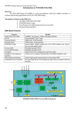
TMS320C5416 DSP Multi Channel Buffered Serial Port [McBSP] Configuration Using Chip
Support Library
1. Connect CRO to the Socket Provided for LINE OUT.
2. Connect a Signal Generator to the LINE IN Socket.
3. Switch on the Signal Generator with a sine wave of frequency 500 Hz.
4. Now Switch on the DSK and Bring Up Code Composer Studio on the PC.
5. Create a new project with name XXXX.pjt.
6. From the File Menu → new → DSP/BIOS Configuration → select “dsk5416.cdb” and save it as
“YYYY.cdb” and add it to the current project.
7. Double click on the “YYYY.cdb” from the project explorer and double click on the “chip support
library” explorer.
8. Double click on the “MCBSP” under the “chip support library” where you can see “MCBSP
Configuration Manager” and “MCBSP Resource Manager”.
9. Right click on the “MCBSP Configuration Manager” and select “Insert mcbspCfg” where you
can see “mcbspCfg0” appearing under “MCBSP Configuration Manager”.
10. Right click on “mcbspCfg0” and select properties where “mcbspCfg0 properties” window
appears.
11. Under “General” property set “Breakpoint Emulation” to “Do Not Stop”.
12. Under “Transmit modes” property set “clock polarity” to “Falling Edge”.
13. Under “Transmit Lengths” property set “Word Length Phase1” to “32-bits” and set
“Words/Frame phase1” to “2”.
14. Under “Receive modes” property set “clock polarity” to “Rising Edge”.
15. Under “Receive Multichannel” property set “Rx Channel Enable” to “All 128 Channels”.
16. Under “Transmit Multichannel” property set “Tx Channel Enable” to “All 128 Channels”.
17. Under the Receive Lengths property set “Word Length Phase1” to “32-bits” and set
“Words/Frame phase1” to “2”.
18. Under the “Sample-Rate Gen” property set “Generator Clock Source” to “BCLKR pin”. Set
“Frame Width” to “32” and “Frame period” to “64”.
19. Select “Apply” and click “O.K”.
20. Select “McBSP2” under the “MCBSP Resource Manager”.
21. Right click on “McBSP2” and select properties where a “McBSP2 Properties” Window appears.
Enable the “Open handle to McBSP” option and “preinitialization“ option. Select “msbspCfg0”
under the “Pre-initialize” pop-up menu and change the “Specify Handle Name” property to
“C54XX_DMA_MCBSP_hMcbsp”. Select “Apply” and click “O.K”.
22. Add the generated “YYYYcfg.cmd” file to the current project.
23. Add the given “mcbsp_io.c” file to the current project which has the main function and calls all
the other necessary routines.
24. View the contents of the generated file “YYYYcfg_c.c” and copy the include header file
‘YYYYcfg.h’ to the “mcbsp_io.c” file.
25. Add the library file “dsk5416f.lib” from the location
“C: CCStudio_v3.1C5400dsk5416libdsk5416f.lib” to the current project
26. Select project → build options → Compiler → Advance and enable the “use Far calls” option.
27. Select project → build options → Compiler → preprocessor and include search path (-i):
“.;$(Install_dir)c5400dsk5416include”.
28. Select project → build options → Linker → Basic include library search path (-i):
“$(Install_dir)c5400dsk5416lib”.

42
29. project→Compile, project→Build, file→Load program and Debug→Run the program.
30. You can notice the input signal of 500 Hz. appearing on the CRO verifying the McBSP
configuration.
mcbsp_io.c:
#include "YYYYcfg.h"
#include <dsk5416.h>
#include <dsk5416_pcm3002.h>
short left_input,right_input;
DSK5416_PCM3002_Config setup = {
0x1ff, // Set-Up Reg 0 - Left channel DAC attenuation
0x1ff, // Set-Up Reg 1 - Right channel DAC attenuation
0x0, // Set-Up Reg 2 - Various ctl e.g. power-down modes
0x0 // Set-Up Reg 3 - Codec data format control
};
void main ()
{
DSK5416_PCM3002_CodecHandle hCodec;
// Initialize the board support library
DSK5416_init();
// Start the codec
hCodec = DSK5416_PCM3002_openCodec(0, &setup);
// Set codec frequency
DSK5416_PCM3002_setFreq(hCodec, 48000);
// Endless loop IO audio codec
while(1){
// Read 16 bits of codec data, loop to retry if data port is busy
while(!DSK5416_PCM3002_read16(hCodec, &left_input));
while(!DSK5416_PCM3002_read16(hCodec, &right_input));
// Write 16 bits to the codec, loop to retry if data port is busy
while(!DSK5416_PCM3002_write16(hCodec, left_input));
while(!DSK5416_PCM3002_write16(hCodec, right_input));
}
}

43
Exp No: 12 Date : _ _/_ _/_ _
GENERATION OF SIGNALS
Aim:
To design and implement a Digital IIR Filter and observe its frequency response.
Equipments needed:
 Host (PC) with windows(95/98/Me/XP/NT/2000).
 TMS320C5416 DSP Starter Kit (DSK).
 Oscilloscope and Function generator.
Flowchart for generation of signals:
Program for Generation of signals:
1. Genration of sine wave:
#include "filtercfg.h"
Int16 left_output;
Int16 right_output;
float sinp = 0;
float cosp = 1;
float sini = 0.0523359562;
float cosi = 0.9986295348;
};
void main ()
{
float st,ct;
Start
Initialize the DSP Board
Set initial Conditions
Determine output and write
output to analog I/O
Stop

44
DSK5416_init();
// Start the codec
while(1)
{
st = sinp*cosi + cosp*sini;
ct = cosp*cosi - sinp*sini;
sinp = st;
cosp = ct;
left_output=32768*sinp;
right_output=left_output;
while(!DSK5416_PCM3002_write16(hCodec, left_output));
while(!DSK5416_PCM3002_write16(hCodec, right_output));
}
}
2. Generation of Triangular wave:
#define PI 3.14159265358979
Int16 left_output;
Int16 right_output;
float sinp[6] = {0,0,0,0,0,0};
float cosp[6] = {1,1,1,1,1,1};
float sini[6] = {0.0523359562, 0.1564344650, 0.2588190451, 0.3583679495, 0.4539904997,
0.5446390350};
float cosi[6] = {0.9986295348, 0.9876883406, 0.9659258263, 0.9335804265, 0.8910065242,
0.8386705679};
};
void main ()
{
int j;
float sp,cp,si,ci,st,ct,temp;
DSK5416_init();
// Start the codec

45
while(1)
{
for(j=0;j<6;j++)
{
sp = sinp[j];
cp = cosp[j];
si = sini[j];
ci = cosi[j];
st = sp*ci + cp*si;
ct = cp*ci - sp*si;
sinp[j] = st;
cosp[j] = ct;
}
temp = 0.5;
for(j=0;j<6;j++)
temp += -4*cosp[j]/(PI*PI*(2*j+1)*(2*j+1));
left_output=32768*temp;
}
}
Result:
Thus sine wave and triangular wave are generated using TMS320c5416 DSK.

46
Exp No: 13 Date : _ _/_ _/_ _
IIR filter Design
Aim:
To design and implement a Digital IIR Filter and observe its frequency response.
Equipments needed:
Flowchart for implementing IIR filter:

47
‘C’ PROGRAM TO IMPLEMENT IIR FILTER:
Int16 left_input;
Int16 left_output;
Int16 right_input;
Int16 right_output;
const signed int filter_Coeff[ ] ={48,48,48, 32767, -30949, 29322};
};
void main ()
{
DSK5416_init();
// Start the codec
DSK5416_PCM3002_setFreq(hCodec,24000);
while(1)
{
left_output=IIR_FILTER(&filter_Coeff , left_input);
}
}
signed int IIR_FILTER(const signed int * h, signed int x1)
{
static signed int x[6] = { 0, 0, 0, 0, 0, 0 }; /* x(n), x(n-1), x(n-2). Must
be static */
static signed int y[6] = { 0, 0, 0, 0, 0, 0 }; /* y(n), y(n-1), y(n-2). Must
be static */
long temp=0;
temp = x1; /* Copy input to temp */
x[0] = (signed int) temp; /* Copy input to x[stages][0] */
temp = ( (long)h[0] * x[0]) ; /* B0 * x(n) */
temp += ( (long)h[1] * x[1]); /* B1/2 * x(n-1) */
temp += ( (long)h[1] * x[1]); /* B1/2 * x(n-1) */
temp += ( (long)h[2] * x[2]); /* B2 * x(n-2) */
temp -= ( (long)h[4] * y[1]); /* A1/2 * y(n-1) */

48
temp -= ( (long)h[4] * y[1]); /* A1/2 * y(n-1) */
temp -= ( (long)h[5] * y[2]); /* A2 * y(n-2) */
/* Divide temp by coefficients[A0] */
temp >>= 15;
if ( temp > 32767 )
{
temp = 32767;
}
else if ( temp < -32767)
{
temp = -32767;
}
y[0] = (short int) ( temp );
/* Shuffle values along one place for next time */
y[2] = y[1]; /* y(n-2) = y(n-1) */
y[1] = y[0]; /* y(n-1) = y(n) */
x[2] = x[1]; /* x(n-2) = x(n-1) */
x[1] = x[0]; /* x(n-1) = x(n) */
/* temp is used as input next time through */
return ((short int)temp*1);
}

49
TABULATION:
Input Voltage ( ) = V
Frequency
in Hz
Output
Voltage ( )
in V
= /
20
in dB

50
Procedure:
 Switch on the DSP board.
 Open the Code Composer Studio.
 Create a new project
 Project " New (File Name. pjt , Eg: Filter.pjt)
 Initialize the McBSP, the DSP board and the on board codec.
“Kindly refer the Topic Configuration of 5416 McBSP using CSL”
 Add the given above .C. source file to the current project(remove mcbsp_io.c source
file from the project if you have already added).
 Connect the speaker jack to the input of the CRO.
 Build the program.
 Load the generated object file(*.out) on to Target board.
 Run the program using F5.
 Observe the waveform that appears on the CRO screen.
Result:
Thus a Digital IIR Filter is designed and implemented and its frequency response is observed.

51
Exp No: 14 Date : _ _/_ _/_ _
FIR filter Design
Aim:
To design and implement a Digital FIR Filter and observe its frequency response.
Equipments needed:
Flowchart for implementing FIR filter:

52
‘C’ PROGRAM TO IMPLEMENT FIR FILTER:
Int16 left_input;
Int16 left_output;
Int16 right_input;
Int16 right_output;
static short in_buffer[100];
float filter_Coeff[] ={-0.000050,-0.000138,0.000198,0.001345,0.002212,-0.000000,-
0.006489,-0.012033,-0.005942,0.016731,0.041539,0.035687,-0.028191,-0.141589,-
0.253270,0.700008,-0.253270,-0.141589,-0.028191,0.035687,0.041539,0.016731,-
0.005942,-0.012033,-0.006489,-0.000000,0.002212,0.001345,0.000198,-0.000138,-
0.000050};
};
void main ()
{
DSK5416_init();
// Start the codec
DSK5416_PCM3002_setFreq(hCodec,8000);
while(1)
{
left_output=FIR_FILTER(&filter_Coeff ,left_input);
}
}
signed int FIR_FILTER(float * h, signed int x)
{
int i=0;
signed long output=0;
in_buffer[0] = x; /* new input at buffer[0] */
for(i=31;i>0;i--)
in_buffer[i] = in_buffer[i-1]; /* shuffle the buffer */
for(i=0;i<32;i++)
output = output + h[i] * in_buffer[i];
return(output);
}

53
TABULATION:
Input Voltage ( ) = V
Frequency
in Hz
Output
Voltage ( )
in V
= /
20
in dB

54
Procedure:
 Switch on the DSP board.
 Open the Code Composer Studio.
 Create a new project
 Project " New (File Name. pjt , Eg: Filter.pjt)
 Initialize the McBSP, the DSP board and the on board codec.
“Kindly refer the Topic Configuration of 5416 McBSP using CSL”
 Add the given above .C. source file to the current project(remove mcbsp_io.c source
file from the project if you have already added).
 Connect the speaker jack to the input of the CRO.
 Build the program.
 Load the generated object file(*.out) on to Target board.
 Run the program using F5.
 Observe the waveform that appears on the CRO screen.
Result:
Thus a Digital FIR Filter is designed and implemented and its frequency response is
observed.

digital signal-processing-lab-manual

More Related Content

What's hot

Viewers also liked

Similar to digital signal-processing-lab-manual

Recently uploaded

digital signal-processing-lab-manual