![EC 313: Adaptive Signal Processing Mayank Awasthi(10531005)
MATLAB Assignment – 1 M.Tech , Communication Systems
IIT Roorkee
Chapter -5, Ques-20
function []= ques20()
%Given
a=.99;
uu=.05;
%Initializing v,u matrices to zero
v=zeros(100,101);
u=zeros(100,101);
%White noise generation with mean =0, variance= 0.02
for i= 1:100
v(i,:)= sqrt(0.02)*randn(1,101);
end
%Generating AR process with variance variance=1 considering 100 independent
%realizations
for i=1:100
u(i,:)=filter(1 ,[1 a] ,v(i,:));
end
for n=1:100
w(1)=0;
for i=1:100
f(n,i)=u(n,i)-w(i)*u(n,i+1);
w(i+1)=w(i)+0.05*u(n,i+1)*f(n,i);
end
end
for i=1:100
for j=1:100
f(i,j)=f(i,j)^2;
end
end
%Ensemble averaging over 100 independent realization of the squared value
%of its output.
for n=1:100
J(n)=mean(f(:,n));
end
%Plotting Learning Curve
plot(J)
end
Mayank Awasthi(10531005), M.Tech , Communication Systems, IIT Roorkee](https://image.slidesharecdn.com/adaptivesignalprocessingsimonhaykins-110530032949-phpapp02/85/Adaptive-signal-processing-simon-haykins-1-320.jpg)

![Chapter -5, Ques-21
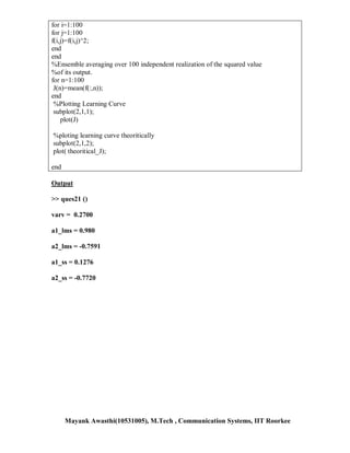
function []= ques21()
%Given
a1= 0.1;
a2= -0.8;
uu=0.05;
varv= 1- (a1*a1)/(1+a2)- (a2*a2) + (a1*a1*a2)/(1+a2)
v=zeros(1,102);
u=zeros(1,102);
%White noise generation with mean =0, variance= vvarv
v= sqrt(varv)*randn(1,102);
%Generating AR process with variance variance=1
u=filter(1 ,[1 a1,a2] ,v);
%Applying the LMS algorithm to calculate a1 and a2
w1(1)=0;
w2(1)=0;
for i=1:100
f(i)=u(i)-w1(i)*u(i+1)-w2(i)*u(i+2);
w1(i+1)=w1(i)+0.05*u(i+1)*f(i);
w2(i+1)=w2(i)+0.05*u(i+2)*f(i);
end
a1_lms= -w1(100)
a2_lms= -w2(100)
%calculating eigen values
eig1= 1- a1/(1+a2);
eig2= 1+ a1/(1+a2);
%maximum step size
uumax= 2/eig2;
%calculating correlation matx and cross correlation matrix
R=[1, -a1/(1+a2); -a1/(1+a2), 1];
r1= -a1/(1+a2);
r2= (a1*a1)/(1+a2)- a2;
p= [r1;r2];
%Calculating optimum weights and minimum mean square error
wo= inv(R)*p;
Jmin= 1-transpose(p)*wo;
%Estimating expected value of weights and variance using small step size theory with
w(0)=0 so we have
v1(1)= -1/sqrt(2)*(a1+a2);
v2(1)= -1/sqrt(2)*(a1-a2);
for n=1:100
val=1;
Mayank Awasthi(10531005), M.Tech , Communication Systems, IIT Roorkee](https://image.slidesharecdn.com/adaptivesignalprocessingsimonhaykins-110530032949-phpapp02/85/Adaptive-signal-processing-simon-haykins-3-320.jpg)
![for j=1:n
val= (1-uu*eig1)*val;
end
meanv1(n)=v1(1)*val;
meansqv1(n)= uu*Jmin/(2-uu*eig1)+ val*val*(v1(1)*v1(1)- uu*Jmin/(2-
uu*eig1));
end
for n=1:100
val=1;
for j=1:n
val= (1-uu*eig2)*val;
end
meanv2(n)=v2(1)*val;
meansqv2(n)= uu*Jmin/(2-uu*eig2)+ val*val*(v2(1)*v2(1)- uu*Jmin/(2-
uu*eig2));
end
for n=1:100
w1(n)= -a1-(meanv1(n)+meanv2(n))/sqrt(2);
w2(n)= -a2-(meanv1(n)-meanv2(n))/sqrt(2);
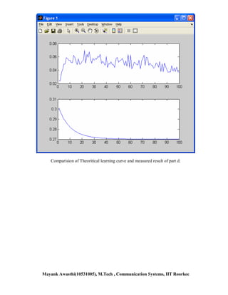
theoritical_J(n)= Jmin + eig1*meansqv1(n)*meansqv1(n) +
eig2*meansqv2(100)*meansqv2(n);
end
expectedvalue_weights=[w1(100);w2(100)];
a1_ss= -w1(100)
a2_ss= -w2(100)
%Generating AR process with variance variance=1 considering 100 independent
%realizations
v=zeros(100,102);
u=zeros(100,102);
%White noise generation with mean =0, variance= 0.02
for i= 1:100
v(i,:)= sqrt(0.02)*randn(1,102);
u(i,:)=filter(1 ,[1 a1,a2] ,v(i,:));
end
for n=1:100
w1(1)=0;
w2(1)=0;
for i=1:100
f(n,i)=u(n,i)-w1(i)*u(n,i+1)-w2(i)*u(n,i+2);
w1(i+1)=w1(i)+0.05*u(n,i+1)*f(n,i);
w2(i+1)=w2(i)+0.05*u(n,i+2)*f(n,i);
end
end
Mayank Awasthi(10531005), M.Tech , Communication Systems, IIT Roorkee](https://image.slidesharecdn.com/adaptivesignalprocessingsimonhaykins-110530032949-phpapp02/85/Adaptive-signal-processing-simon-haykins-4-320.jpg)
![Chapter-5 Ques 21- Part c
function []= ques21()
%Given
a1= 0.1;
a2= -0.8;
varv= 1- (a1*a1)/(1+a2)- (a2*a2) + (a1*a1*a2)/(1+a2);
v=zeros(1,102);
u=zeros(1,102);
%White noise generation with mean =0, variance= vvarv
v= sqrt(varv)*randn(1,102);
%Generating AR process with variance variance=1
u=filter(1 ,[1 a1,a2] ,v);
w1(1)=0;
w2(1)=0;
for i=1:100
f(i)=u(i)-w1(i)*u(i+1)-w2(i)*u(i+2);
w1(i+1)=w1(i)+0.05*u(i+1)*f(i);
w2(i+1)=w2(i)+0.05*u(i+2)*f(i);
e1(i)= -a1-w1(i);
e2(i)= -a2-w2(i);
end
Fs = 32e3;
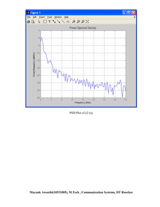
Pxx = periodogram(f);
Hpsd = dspdata.psd(Pxx,'Fs',Fs); % Create a PSD data object.
plot(Hpsd); % Plot the PSD.
Pxx = periodogram(e1);
Hpsd = dspdata.psd(Pxx,'Fs',Fs); % Create a PSD data object.
plot(Hpsd); % Plot the PSD.
Pxx = periodogram(e2);
Hpsd = dspdata.psd(Pxx,'Fs',Fs); % Create a PSD data object.
plot(Hpsd); % Plot the PSD.
End
Mayank Awasthi(10531005), M.Tech , Communication Systems, IIT Roorkee](https://image.slidesharecdn.com/adaptivesignalprocessingsimonhaykins-110530032949-phpapp02/85/Adaptive-signal-processing-simon-haykins-7-320.jpg)


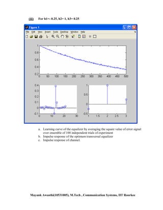
![Chapter -5, Ques-22
function []= ques22(h1,h2,h3)
iter=500; %no pf iterations
M=21; %no of tap inputs
P=100; %no of independent experiments
uu=0.001; %learning parameter
h=[h1 h2 h3]; %channel impulse response
D1=1; %channel impulse response is symmetric about n=1
D2=(M-1)/2;
D=D1+D2; %total delay
for j=1:P
%Generating Bernoulli sequence
x=sign(rand(1,530)-0.5);
%channel output
u1 =conv(x,h);
v=sqrt(0.01)*randn(1,length(u1));
%adding AWGN noise with channel output
u=u1+v;
%Applying LMS Algoritm
w=zeros(1,M); %initializing weight vector
for i=1:iter
f(j,i) = x(D+i)- w*transpose(u(i:M-1+i));
w= w+ uu*u(i:M-1+i)*f(j,i);
end
end
subplot(2,2,3);
stem(w); %Plotting the weight vector
subplot(2,2,4);
stem(h); %Plotting the impuse response of channel
%Ensemble averaging over 100 independent realization of the squared value
%of its output.
for j=1:P
f(j,:)= f(j,:).^2;
end
for n=1:iter
J(n)=mean(f(:,n));
End
%Plotting the learning curve
subplot(2,2,1:2);
plot(J);
end
Mayank Awasthi(10531005), M.Tech , Communication Systems, IIT Roorkee](https://image.slidesharecdn.com/adaptivesignalprocessingsimonhaykins-110530032949-phpapp02/85/Adaptive-signal-processing-simon-haykins-11-320.jpg)
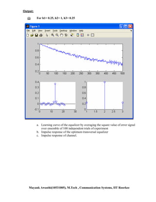

This document contains MATLAB code for an assignment on adaptive signal processing. It includes code to: 1. Generate autoregressive processes and apply the LMS algorithm to estimate filter coefficients. 2. Compare the theoretical and experimental learning curves for an adaptive filter estimating coefficients of an AR(2) process. 3. Estimate the impulse response of a channel equalizer using LMS adaptation and observe the learning curve and estimated taps. The code contains comments explaining the steps and outputs learning curves, estimated filter weights, and channel impulse responses for analysis. It was written by Mayank Awasthi, an IIT Roorkee student, for an assignment on adaptive filtering techniques.