The document contains MATLAB scripts for generating and plotting various discrete-time signals, including unit samples, unit steps, real and complex exponentials, and sinusoidal sequences. It also illustrates the noncommutativity of folding and shifting operations on discrete signals, showcasing the effects through plots. Additionally, it presents techniques for creating periodic signals using specific MATLAB functions.
![CHAPTER 2
Discrete-Time Signals and Systems
Tutorial Problems
1. (a) MATLAB script:
% P0201a: Generate and plot unit sample
close all; clc
n = -20:40; % specifiy support of signal
deltan = zeros(1,length(n)); % define signal
deltan(n==0)=1;
% Plot:
hf = figconfg(’P0201a’,’small’);
stem(n,deltan,’fill’)
axis([min(n)-1,max(n)+1,min(deltan)-0.2,max(deltan)+0.2])
xlabel(’n’,’fontsize’,LFS); ylabel(’delta[n]’,’fontsize’,LFS);
title(’Unit Sample delta[n]’,’fontsize’,TFS)
−20 −10 0 10 20 30 40
−0.2
0
0.2
0.4
0.6
0.8
1
n
δ[n]
Unit Sample δ[n]
FIGURE 2.1: unit sample δ[n].
1
Applied Digital Signal Processing 1st Edition Manolakis Solutions Manual
Full Download: http://alibabadownload.com/product/applied-digital-signal-processing-1st-edition-manolakis-solutions-manual/
This sample only, Download all chapters at: alibabadownload.com](https://image.slidesharecdn.com/applied-digital-signal-processing-1st-edition-manolakis-solutions-manual-190422092224/85/Applied-Digital-Signal-Processing-1st-Edition-Manolakis-Solutions-Manual-1-320.jpg)
![CHAPTER 2
Discrete-Time Signals and Systems
Tutorial Problems
1. (a) MATLAB script:
% P0201a: Generate and plot unit sample
close all; clc
n = -20:40; % specifiy support of signal
deltan = zeros(1,length(n)); % define signal
deltan(n==0)=1;
% Plot:
hf = figconfg(’P0201a’,’small’);
stem(n,deltan,’fill’)
axis([min(n)-1,max(n)+1,min(deltan)-0.2,max(deltan)+0.2])
xlabel(’n’,’fontsize’,LFS); ylabel(’delta[n]’,’fontsize’,LFS);
title(’Unit Sample delta[n]’,’fontsize’,TFS)
−20 −10 0 10 20 30 40
−0.2
0
0.2
0.4
0.6
0.8
1
n
δ[n]
Unit Sample δ[n]
FIGURE 2.1: unit sample δ[n].
1
Applied Digital Signal Processing 1st Edition Manolakis Solutions Manual
Full Download: http://alibabadownload.com/product/applied-digital-signal-processing-1st-edition-manolakis-solutions-manual/
This sample only, Download all chapters at: alibabadownload.com](https://image.slidesharecdn.com/applied-digital-signal-processing-1st-edition-manolakis-solutions-manual-190422092224/75/Applied-Digital-Signal-Processing-1st-Edition-Manolakis-Solutions-Manual-1-2048.jpg)
![CHAPTER 2. Discrete-Time Signals and Systems 2
(b) MATLAB script:
% P0201b: Generate and plot unit step sequence
close all; clc
n = -20:40; % specifiy support of signal
un = zeros(1,length(n)); % define signal
un(n>=0)=1;
% Plot:
hf = figconfg(’P0201b’,’small’);
stem(n,un,’fill’)
axis([min(n)-1,max(n)+1,min(un)-0.2,max(un)+0.2])
xlabel(’n’,’fontsize’,LFS); ylabel(’u[n]’,’fontsize’,LFS);
title(’Unit Step u[n]’,’fontsize’,TFS)
−20 −10 0 10 20 30 40
−0.2
0
0.2
0.4
0.6
0.8
1
n
u[n]
Unit Step u[n]
FIGURE 2.2: unit step u[n].
(c) MATLAB script:
% P0201c: Generate and plot real exponential sequence
close all; clc
n = -20:40; % specifiy support of signal
x1n = 0.8.^n; % define signal
% Plot:
hf = figconfg(’P0201c’,’small’);
stem(n,x1n,’fill’)
axis([min(n)-1,max(n)+1,min(x1n)-5,max(x1n)+5])
xlabel(’n’,’fontsize’,LFS); ylabel(’x_1[n]’,’fontsize’,LFS);
title(’Real Exponential Sequence x_1[n]’,’fontsize’,TFS)
(d) MATLAB script:](https://image.slidesharecdn.com/applied-digital-signal-processing-1st-edition-manolakis-solutions-manual-190422092224/85/Applied-Digital-Signal-Processing-1st-Edition-Manolakis-Solutions-Manual-2-320.jpg)
![CHAPTER 2. Discrete-Time Signals and Systems 3
−20 −10 0 10 20 30 40
0
20
40
60
80
n
x
1
[n]
Real Exponential Sequence x
1
[n]
FIGURE 2.3: real exponential signal x1[n] = (0.80)n.
% P0201d: Generate and plot complex exponential sequence
close all; clc
n = -20:40; % specifiy support of signal
x2n = (0.9*exp(j*pi/10)).^n; % define signal
x2n_r = real(x2n); % real part
x2n_i = imag(x2n); % imaginary part
x2n_m = abs(x2n); % magnitude part
x2n_p = angle(x2n); % phase part
% Plot:
hf = figconfg(’P0201d’);
subplot(2,2,1)
stem(n,x2n_r,’fill’)
axis([min(n)-1,max(n)+1,min(x2n_r)-1,max(x2n_r)+1])
xlabel(’n’,’fontsize’,LFS); ylabel(’Re{x_2[n]}’,’fontsize’,LFS);
title(’Real Part of Sequence x_2[n]’,’fontsize’,TFS)
subplot(2,2,2)
stem(n,x2n_i,’fill’)
axis([min(n)-1,max(n)+1,min(x2n_i)-1,max(x2n_i)+1])
xlabel(’n’,’fontsize’,LFS); ylabel(’Im{x_2[n]}’,’fontsize’,LFS);
title(’Imaginary Part of Sequence x_2[n]’,’fontsize’,TFS)
subplot(2,2,3)
stem(n,x2n_m,’fill’)
axis([min(n)-1,max(n)+1,min(x2n_m)-1,max(x2n_m)+1])
xlabel(’n’,’fontsize’,LFS); ylabel(’|x_2[n]|’,’fontsize’,LFS);
title(’Magnitude of Sequence x_2[n]’,’fontsize’,TFS)
subplot(2,2,4)](https://image.slidesharecdn.com/applied-digital-signal-processing-1st-edition-manolakis-solutions-manual-190422092224/85/Applied-Digital-Signal-Processing-1st-Edition-Manolakis-Solutions-Manual-3-320.jpg)
![CHAPTER 2. Discrete-Time Signals and Systems 4
stem(n,x2n_p,’fill’)
axis([min(n)-1,max(n)+1,min(x2n_p)-1,max(x2n_p)+1])
xlabel(’n’,’fontsize’,LFS); ylabel(’phi(x_2[n])’,’fontsize’,LFS);
title(’Phase of Sequence x_2[n]’,’fontsize’,TFS)
−20 −10 0 10 20 30 40
−4
−2
0
2
4
6
8
n
Re{x2
[n]}
Real Part of Sequence x
2
[n]
−20 −10 0 10 20 30 40
−2
0
2
4
6
n
Im{x2
[n]}
Imaginary Part of Sequence x
2
[n]
−20 −10 0 10 20 30 40
0
2
4
6
8
n
|x2
[n]|
Magnitude of Sequence x
2
[n]
−20 −10 0 10 20 30 40
−4
−2
0
2
4
n
φ(x2
[n])
Phase of Sequence x
2
[n]
FIGURE 2.4: complex exponential signal x2[n] = (0.9ejπ/10)n.
(e) MATLAB script:
% P0201e: Generate and plot real sinusoidal sequence
close all; clc
n = -20:40; % specifiy support of signal
x3n = 2*cos(2*pi*0.3*n+pi/3); % define signal
% Plot:
hf = figconfg(’P0201e’,’small’);
stem(n,x3n,’fill’)
axis([min(n)-1,max(n)+1,min(x3n)-0.5,max(x3n)+0.5])
xlabel(’n’,’fontsize’,LFS); ylabel(’x_3[n]’,’fontsize’,LFS);
title(’Real Sinusoidal Sequence x_3[n]’,’fontsize’,TFS)](https://image.slidesharecdn.com/applied-digital-signal-processing-1st-edition-manolakis-solutions-manual-190422092224/85/Applied-Digital-Signal-Processing-1st-Edition-Manolakis-Solutions-Manual-4-320.jpg)
![CHAPTER 2. Discrete-Time Signals and Systems 5
−20 −10 0 10 20 30 40
−2
−1
0
1
2
n
x
3
[n]
Real Sinusoidal Sequence x
3
[n]
FIGURE 2.5: sinusoidal sequence x3[n] = 2 cos[2π(0.3)n + π/3].
2. MATLAB script:
% P0202: Illustrate the noncommutativity of folding and shifting
close all; clc
nx = 0:4; % specify the support
x = 5:-1:1; % specify sequence
n0 = 2;
% (a) First folding, then shifting
[y1 ny1] = fold(x,nx);
[y1 ny1] = shift(y1,ny1,-n0);
% (b) First shifting, then folding
[y2 ny2] = shift(x,nx,-n0);
[y2 ny2] = fold(y2,ny2);
% Plot
hf = figconfg(’P0202’);
xylimit = [min([nx(1),ny1(1),ny2(1)])-1,max([nx(end),ny1(end)...
,ny2(end)])+1,min(x)-1,max(x)+1];
subplot(3,1,1)
stem(nx,x,’fill’)
axis(xylimit)
ylabel(’x[n]’,’fontsize’,LFS); title(’x[n]’,’fontsize’,TFS);
set(gca,’Xtick’,xylimit(1):xylimit(2))
subplot(3,1,2)
stem(ny1,y1,’fill’)
axis(xylimit)
ylabel(’y_1[n]’,’fontsize’,LFS);](https://image.slidesharecdn.com/applied-digital-signal-processing-1st-edition-manolakis-solutions-manual-190422092224/85/Applied-Digital-Signal-Processing-1st-Edition-Manolakis-Solutions-Manual-5-320.jpg)
![CHAPTER 2. Discrete-Time Signals and Systems 6
title(’y_1[n]: Folding and Shifting’,’fontsize’,TFS)
set(gca,’Xtick’,xylimit(1):xylimit(2))
subplot(3,1,3)
stem(ny2,y2,’fill’)
axis(xylimit)
xlabel(’n’,’fontsize’,LFS); ylabel(’y_2[n]’,’fontsize’,LFS);
title(’y_2[n]: Shifting and Folding’,’fontsize’,TFS)
set(gca,’Xtick’,xylimit(1):xylimit(2))
−7 −6 −5 −4 −3 −2 −1 0 1 2 3 4 5
0
5
x[n]
x[n]
−7 −6 −5 −4 −3 −2 −1 0 1 2 3 4 5
0
5
y1
[n]
y
1
[n]: Folding and Shifting
−7 −6 −5 −4 −3 −2 −1 0 1 2 3 4 5
0
5
n
y2
[n]
y
2
[n]: Shifting and Folding
FIGURE 2.6: Illustrating noncommunativity of folding and shifting operations.
Comments:
From the plot, we can see y1[n] and y2[n] are different. Indeed, y1[n] repre-
sents the correct x[2 − n] signal while y2[n] represents signal x[−n − 2].
3. (a) x[−n] = {4, 4, 4, 4, 4
↑
, 3, 2, 1, 0, −1}
x[n − 3] = {−1, 0, 1
↑
, 2, 3, 4, 4, 4, 4, 4}
x[n + 2] = {−1, 0, 1, 2, 3, 4, 4, 4
↑
, 4, 4}](https://image.slidesharecdn.com/applied-digital-signal-processing-1st-edition-manolakis-solutions-manual-190422092224/85/Applied-Digital-Signal-Processing-1st-Edition-Manolakis-Solutions-Manual-6-320.jpg)
![CHAPTER 2. Discrete-Time Signals and Systems 7
(b) see part (c)
(c) MATLAB script:
% P0203bc: Illustrate the folding and shifting effect
close all; clc
nx = -5:4; % specify support
x = [-1:4,4*ones(1,4)]; % define sequence
[y1 ny1] = fold(x,nx); % folding
[y2 ny2] = shift(x,nx,-3); % right-shifting
[y3 ny3] = shift(x,nx,2); % left-shifting
% Plot
hf = figconfg(’P0203’);
xylimit = [min([nx(1),ny1(1),ny2(1),ny3(1)])-1,max([nx(end),...
ny1(end),ny2(end),ny2(end)])+1,min(x)-1,max(x)+1];
subplot(4,1,1)
stem(nx,x,’fill’); axis(xylimit)
ylabel(’x[n]’,’fontsize’,LFS); title(’x[n]’,’fontsize’,TFS);
set(gca,’Xtick’,xylimit(1):xylimit(2))
subplot(4,1,2)
stem(ny1,y1,’fill’); axis(xylimit)
ylabel(’x[-n]’,’fontsize’,LFS); title(’x[-n]’,’fontsize’,TFS)
set(gca,’Xtick’,xylimit(1):xylimit(2))
subplot(4,1,3)
stem(ny2,y2,’fill’); axis(xylimit)
ylabel(’x[n-3]’,’fontsize’,LFS); title(’x[n-3]’,’fontsize’,TFS);
set(gca,’Xtick’,xylimit(1):xylimit(2))
subplot(4,1,4)
stem(ny3,y3,’fill’); axis(xylimit)
xlabel(’n’,’fontsize’,LFS); ylabel(’x[n+2]’,’fontsize’,LFS);
title(’x[n+2]’,’fontsize’,TFS)
set(gca,’Xtick’,xylimit(1):xylimit(2))
4. MATLAB script:
% P0204: Illustrate the using of repmat, persegen and pulstran
% to generate periodic signal
close all; clc
n = 0:9; % specify support
x = [ones(1,4),zeros(1,6)]; % sequence 1
% x = cos(0.1*pi*n); % sequence 2](https://image.slidesharecdn.com/applied-digital-signal-processing-1st-edition-manolakis-solutions-manual-190422092224/85/Applied-Digital-Signal-Processing-1st-Edition-Manolakis-Solutions-Manual-7-320.jpg)
![CHAPTER 2. Discrete-Time Signals and Systems 8
−8 −7 −6 −5 −4 −3 −2 −1 0 1 2 3 4 5 6 7 8
−2
0
2
4x[n]
x[n]
−8 −7 −6 −5 −4 −3 −2 −1 0 1 2 3 4 5 6 7 8
−2
0
2
4
x[−n]
x[−n]
−8 −7 −6 −5 −4 −3 −2 −1 0 1 2 3 4 5 6 7 8
−2
0
2
4
x[n−3]
x[n−3]
−8 −7 −6 −5 −4 −3 −2 −1 0 1 2 3 4 5 6 7 8
−2
0
2
4
n
x[n+2]
x[n+2]
FIGURE 2.7: Illustrating folding and shifting operations.
% x = 0.8.^n; % sequence 3
Np = 5; % number of periods
xp1 = repmat(x,1,Np);
nxp1 = n(1):Np*length(x)-1;
[xp2 nxp2] = persegen(x,length(x),Np*length(x),n(1));
xp3 = pulstran(nxp1,(0:Np-1)’*length(x),x);
%Plot
hf = figconfg(’P0204’);
xylimit = [-1,nxp1(end)+1,min(x)-1,max(x)+1];
subplot(3,1,1)
stem(nxp1,xp1,’fill’); axis(xylimit)
ylabel(’x_p[n]’,’fontsize’,LFS);
title(’Function ’’repmat’’’,’fontsize’,TFS);
subplot(3,1,2)
stem(nxp2,xp2,’fill’); axis(xylimit)
ylabel(’x_p[n]’,’fontsize’,LFS);](https://image.slidesharecdn.com/applied-digital-signal-processing-1st-edition-manolakis-solutions-manual-190422092224/85/Applied-Digital-Signal-Processing-1st-Edition-Manolakis-Solutions-Manual-8-320.jpg)
![CHAPTER 2. Discrete-Time Signals and Systems 9
title(’Function ’’persegen’’’,’fontsize’,TFS)
subplot(3,1,3)
stem(nxp1,xp3,’fill’); axis(xylimit)
xlabel(’n’,’fontsize’,LFS); ylabel(’x_p[n]’,’fontsize’,LFS);
title(’Function ’’pulstran’’’,’fontsize’,TFS)
0 5 10 15 20 25 30 35 40 45 50
−1
0
1
2
xp
[n]
Function ’repmat’
0 5 10 15 20 25 30 35 40 45 50
−1
0
1
2
xp
[n]
Function ’persegen’
0 5 10 15 20 25 30 35 40 45 50
−1
0
1
2
n
xp
[n]
Function ’pulstran’
FIGURE 2.8: Periodically expanding sequence {1 1 1 1 0 0 0 0 0 0}.](https://image.slidesharecdn.com/applied-digital-signal-processing-1st-edition-manolakis-solutions-manual-190422092224/85/Applied-Digital-Signal-Processing-1st-Edition-Manolakis-Solutions-Manual-9-320.jpg)
![CHAPTER 2. Discrete-Time Signals and Systems 10
0 5 10 15 20 25 30 35 40 45 50
−1
0
1
2
x
p
[n]
Function ’repmat’
0 5 10 15 20 25 30 35 40 45 50
−1
0
1
2
x
p
[n]
Function ’persegen’
0 5 10 15 20 25 30 35 40 45 50
−1
0
1
2
n
x
p
[n]
Function ’pulstran’
FIGURE 2.9: Periodically expanding sequence cos(0.1πn), 0 ≤ n ≤ 9.
0 5 10 15 20 25 30 35 40 45 50
0
1
2
xp
[n]
Function ’repmat’
0 5 10 15 20 25 30 35 40 45 50
0
1
2
xp
[n]
Function ’persegen’
0 5 10 15 20 25 30 35 40 45 50
0
1
2
n
xp
[n]
Function ’pulstran’
FIGURE 2.10: Periodically expanding sequence 0.8n, 0 ≤ n ≤ 9.](https://image.slidesharecdn.com/applied-digital-signal-processing-1st-edition-manolakis-solutions-manual-190422092224/85/Applied-Digital-Signal-Processing-1st-Edition-Manolakis-Solutions-Manual-10-320.jpg)
![CHAPTER 2. Discrete-Time Signals and Systems 11
5. (a) Proof: If the sinusoidal signal cos(ω0n + θ0) is periodic in n, we need
to find a period Np that satisfy cos(ω0n+θ0) = cos(ω0n+ω0Np +θ0)
for every n. Since f0
ω0
2π is a rational number, we can substitute ω0 =
2πf0 = 2πM
N into the previous periodic condition to have cos(2πM
N n+
θ0) = cos(2πM
N n + 2πM
N Np + θ0). No matter what integers M and N
take, Np = N is a period of the sinusoidal signal.
(b) The sequence is NOT periodic.
(c) The sequence is periodic with fundamental period N = 10. N can
be interpreted as period and M is the number of repetitions the corre-
sponding continuous signal repeats itself.
−20 −15 −10 −5 0 5 10 15 20
−1
−0.5
0
0.5
1
n
x1
[n]
Nonperiodic Sequence
−20 −15 −10 −5 0 5 10 15 20
−1
−0.5
0
0.5
1
n
x2
[n]
Periodic Sequence
FIGURE 2.11: Illustrating the periodicity condition of sinusoidal signals.
MATLAB script:
% P0205: Illustrates the condition for periodicity of discrete
% sinusoidal sequence
close all; clc
% Part (b): Nonperiodic](https://image.slidesharecdn.com/applied-digital-signal-processing-1st-edition-manolakis-solutions-manual-190422092224/85/Applied-Digital-Signal-Processing-1st-Edition-Manolakis-Solutions-Manual-11-320.jpg)
![CHAPTER 2. Discrete-Time Signals and Systems 12
n = -20:20; % support
w1 = 0.1; % angular frequency
x1 = cos(w1*n-pi/5);
% Part (c): Periodic
w2 = 0.1*pi; % angular frequency
x2 = cos(w2*n-pi/5);
%Plot
hf = figconfg(’P0205’);
xylimit = [n(1)-1,n(end)+1,min(x1)-0.5,max(x1)+0.5];
subplot(2,1,1)
stem(n,x1,’fill’); axis(xylimit)
xlabel(’n’,’fontsize’,LFS); ylabel(’x_1[n]’,’fontsize’,LFS);
title(’Nonperiodic Sequence’,’fontsize’,TFS);
% set(gca,’Xtick’,xylimit(1):xylimit(2))
subplot(2,1,2)
stem(n,x2,’fill’); axis(xylimit)
xlabel(’n’,’fontsize’,LFS); ylabel(’x_2[n]’,’fontsize’,LFS);
title(’Periodic Sequence’,’fontsize’,TFS)
6. MATLAB script:
% P0206: Investigates the effect of downsampling using
% audio file ’handel’
close all; clc
load(’handel.mat’)
n = 1:length(y);
% Part (a): original sampling rate
sound(y,Fs); pause(1)
% Part (b): downsampling by a factor of two
y_ds2_ind = mod(n,2)==1;
sound(y(y_ds2_ind),Fs/2); pause(1)
% Part (c): downsampling by a factor of four
y_ds4_ind = mod(n,4)==1;
sound(y(y_ds4_ind),Fs/4)
% save the sound file
wavwrite(y(y_ds4_ind),Fs/4,’handel_ds4’)
7. Comments: The first system is NOT time-invariant but the second system is
time invariant.
MATLAB script:](https://image.slidesharecdn.com/applied-digital-signal-processing-1st-edition-manolakis-solutions-manual-190422092224/85/Applied-Digital-Signal-Processing-1st-Edition-Manolakis-Solutions-Manual-12-320.jpg)
![CHAPTER 2. Discrete-Time Signals and Systems 13
0 2 4 6 8 10 12 14 16 18 20
0
0.2
0.4
0.6
0.8
1
n
y1
[n]
y
1
[n]
0 2 4 6 8 10 12 14 16 18 20
0
0.2
0.4
0.6
0.8
1
n
y2
[n]
y
2
[n]
FIGURE 2.12: System responses with respect to input signal x[n] = δ[n].
% P0207: Compute and plot sequence defined by difference equations
close all; clc
n = 0:20; % define support
yi = 0; % zero initial condition
xn = delta(n(1),0,n(end))’; % input 1
% xn = delta(n(1),5,n(end))’; % input 2
% Compute sequence 1:
yn1 = zeros(1,length(n));
yn1(1) = n(1)/(n(1)+1)*yi+xn(1);
for ii = 2:length(n)
yn1(ii) = n(ii)/(n(ii)+1)*yn1(ii-1)+xn(ii);
end
% Compute sequence 2:
yn2 = filter(1,[1,-0.9],xn);
%Plot
hf = figconfg(’P0207’);](https://image.slidesharecdn.com/applied-digital-signal-processing-1st-edition-manolakis-solutions-manual-190422092224/85/Applied-Digital-Signal-Processing-1st-Edition-Manolakis-Solutions-Manual-13-320.jpg)
![CHAPTER 2. Discrete-Time Signals and Systems 14
0 2 4 6 8 10 12 14 16 18 20
0
0.5
1
n
y1
[n]
y
1
[n]
0 2 4 6 8 10 12 14 16 18 20
0
0.5
1
n
y2
[n]
y
2
[n]
FIGURE 2.13: System responses with respect to input signal x[n] = δ[n − 5].
xylimit = [n(1)-1,n(end)+1,min(yn1)-0.2,max(yn1)+0.2];
subplot(2,1,1)
stem(n,yn1,’fill’); axis(xylimit)
xlabel(’n’,’fontsize’,LFS); ylabel(’y_1[n]’,’fontsize’,LFS);
title(’y_1[n]’,’fontsize’,TFS);
subplot(2,1,2)
stem(n,yn2,’fill’); axis(xylimit)
xlabel(’n’,’fontsize’,LFS); ylabel(’y_2[n]’,’fontsize’,LFS);
title(’y_2[n]’,’fontsize’,TFS)
8. (a)
y[n] =
1
5
(x[n] + x[n − 1] + x[n − 2] + x[n − 3] + x[n − 4])
(b)
h[n] = u[n] − u[n − 5]](https://image.slidesharecdn.com/applied-digital-signal-processing-1st-edition-manolakis-solutions-manual-190422092224/85/Applied-Digital-Signal-Processing-1st-Edition-Manolakis-Solutions-Manual-14-320.jpg)
![CHAPTER 2. Discrete-Time Signals and Systems 15
0 5 10 15 20
−0.1
0
0.1
0.2
0.3
n
h[n]
5−Point Moving Average Filter Impulse Response
FIGURE 2.14: Impulse response of a 5-point moving average filter.
(c) Block diagram.
x[n]
y[n]
0.2 0.2
z
−1
0.2
z
−1
0.2
z
−1
0.2
z
−1
FIGURE 2.15: Block diagram of a 5-point moving average filter.
MATLAB script:
% P0208: Plot the 5-point moving average filter
% y[n] = 1/5*(x[n]+x[n-1]+x[n-2]+x[n-3]+x[n-4]);
close all; clc
n = 0:20;
xn = delta(n(1),0,n(end))’;
hn = filter(ones(1,5)/5,1,xn);
%Plot
hf = figconfg(’P0208’,’small’);
xylimit = [n(1)-1,n(end)+1,min(hn)-0.1,max(hn)+0.1];
stem(n,hn,’fill’); axis(xylimit)](https://image.slidesharecdn.com/applied-digital-signal-processing-1st-edition-manolakis-solutions-manual-190422092224/85/Applied-Digital-Signal-Processing-1st-Edition-Manolakis-Solutions-Manual-15-320.jpg)
![CHAPTER 2. Discrete-Time Signals and Systems 16
xlabel(’n’,’fontsize’,LFS); ylabel(’h[n]’,’fontsize’,LFS);
title(’5-Point Moving Average Filter Impulse Response’,...
’fontsize’,TFS);
9. (a) Proof:
∞
n=0
an
= 1 + a + a2
+ · · ·
a
∞
n=0
an
= a + a2
+ a3
+ · · ·
(1 − a)
∞
n=0
an
= 1 + (a − a) + (a2
− a2
) + · · · + (a∞
− a∞
)
(1 − a)
∞
n=0
an
= 1 + 0 + 0 + · · · + 0
∞
n=0
an
=
1
1 − a
(b) Proof:
N−1
n=0
an
=
∞
n=0
an
−
∞
n=N
an
=
∞
n=0
an
− aN
∞
n=0
an
Substituting the result in part (a), we have
N−1
n=0
an
= (1 − aN
)
∞
n=0
an
=
1 − aN
1 − a
10. (a) Solution:
x[−m] = {−1, 2, 3, 1
↑
}
x[3 − m] = {−1
↑
, 2, 3, , 1}
h[m] = {2
↑
, 2(0.8)1
, 2(0.8)2
, 2(0.8)3
, 2(0.8)4
, 2(0.8)5
, 2(0.8)6
}
x[3 − m] ∗ h[m] = {−2
↑
, 4(0.8)1
, 6(0.8)2
, 2(0.8)3
}
y[3] =
3
m=0
x[3 − m] ∗ h[m] = 6.064](https://image.slidesharecdn.com/applied-digital-signal-processing-1st-edition-manolakis-solutions-manual-190422092224/85/Applied-Digital-Signal-Processing-1st-Edition-Manolakis-Solutions-Manual-16-320.jpg)
![CHAPTER 2. Discrete-Time Signals and Systems 17
(b) MATLAB script:
% P0210: Graphically illustrate the convolution sum
close all; clc
nx = 0:3;
x = [1,3,2,-1]; % input sequence
nh = 0:6;
h = 2*(0.8).^nh; % impulse response
nxf = fliplr(-nx); xf = fliplr(x); %folding
nxfs = nxf+3; % left shifting
[y1 y2 n] = timealign(xf,nxfs,h,nh);
y = y1.*y2;
y3 = sum(y);
%Plot
hf = figconfg(’P0210’);
subplot(5,1,1)
stem(nx,x,’fill’)
axis([-4 7 min(x)-1 max(x)+1])
ylabel(’x[k]’,’fontsize’,LFS);
subplot(5,1,2)
stem(nh,h,’fill’)
axis([-4 7 min(h)-1 max(h)+1])
ylabel(’h[k]’,’fontsize’,LFS);
subplot(5,1,3)
stem(nxf,xf,’fill’)
axis([-4 7 min(x)-1 max(x)+1])
ylabel(’x[-k]’,’fontsize’,LFS);
subplot(5,1,4)
stem(nxfs,xf,’fill’)
axis([-4 7 min(x)-1 max(x)+1])
ylabel(’x[-k+3]’,’fontsize’,LFS);
subplot(5,1,5)
stem(n,y,’fill’)
axis([-4 7 min(y)-1 max(y)+1])
xlabel(’k’,’fontsize’,LFS);
ylabel(’h[k]*x[-k+3]’,’fontsize’,LFS);](https://image.slidesharecdn.com/applied-digital-signal-processing-1st-edition-manolakis-solutions-manual-190422092224/85/Applied-Digital-Signal-Processing-1st-Edition-Manolakis-Solutions-Manual-17-320.jpg)
![CHAPTER 2. Discrete-Time Signals and Systems 18
−4 −3 −2 −1 0 1 2 3 4 5 6 7
−2
0
2
4
x[k]
−4 −3 −2 −1 0 1 2 3 4 5 6 7
0
1
2
3
h[k]
−4 −3 −2 −1 0 1 2 3 4 5 6 7
−2
0
2
4
x[−k]
−4 −3 −2 −1 0 1 2 3 4 5 6 7
−2
0
2
4
x[−k+3]
−4 −3 −2 −1 0 1 2 3 4 5 6 7
−2
0
2
4
k
h[k]*x[−k+3]
FIGURE 2.16: Graphically illustration of convolution as a superposition of scaled
and scaled replicas.](https://image.slidesharecdn.com/applied-digital-signal-processing-1st-edition-manolakis-solutions-manual-190422092224/85/Applied-Digital-Signal-Processing-1st-Edition-Manolakis-Solutions-Manual-18-320.jpg)
![CHAPTER 2. Discrete-Time Signals and Systems 19
11. Comments: The step responses of the two equivalent system representations
are equal.
0 2 4 6
−1
0
1
2
3
n
h[n]
System h[n]
−1 0 1 2 3 4 5
−1
0
1
2
3
n
u[n]
Unit Step u[n]
0 2 4 6 8 10
2
4
6
8
n
y1
[n]
Step Response of System I
0 2 4 6 8 10
2
4
6
8
n
y2
[n]
Step Response of System II
FIGURE 2.17: Illustrating equivalent system representation.
MATLAB script:
% P0211: Illustrating the combination of parallel and
% series systems
close all; clc
n1 = 0:4;
h1 = ones(1,5);
h2 = [1 -1 -1 -1 1];
n2 = 0:2;
h3 = ones(1,3);
[h n] = conv0(h1+h2,n1,h3,n2);
un = unitstep(n1(1),0,n1(end));
[ytemp1 nyt] = conv0(h1,n1,un,n1);
ytemp2 = conv(h2,un);](https://image.slidesharecdn.com/applied-digital-signal-processing-1st-edition-manolakis-solutions-manual-190422092224/85/Applied-Digital-Signal-Processing-1st-Edition-Manolakis-Solutions-Manual-19-320.jpg)
![CHAPTER 2. Discrete-Time Signals and Systems 20
[y1 ny1] = conv0(h3,n2,ytemp1+ytemp2,nyt);
[y2 ny2] = conv0(h,n,un,n1);
%Plot
hf = figconfg(’P0211’);
subplot(2,2,1)
stem(n,h,’fill’)
axis([n(1)-1 n(end)+1 min(h)-1 max(h)+1])
xlabel(’n’,’fontsize’,LFS);
ylabel(’h[n]’,’fontsize’,LFS);
title(’System h[n]’,’fontsize’,TFS);
subplot(2,2,2)
stem(n1,un,’fill’)
axis([n1(1)-1 n1(end)+1 min(h)-1 max(h)+1])
xlabel(’n’,’fontsize’,LFS);
ylabel(’u[n]’,’fontsize’,LFS);
title(’Unit Step u[n]’,’fontsize’,TFS);
subplot(2,2,3)
stem(ny1,y1,’fill’)
axis([ny1(1)-1 ny1(end)+1 min(y1)-1 max(y1)+1])
xlabel(’n’,’fontsize’,LFS);
ylabel(’y_1[n]’,’fontsize’,LFS);
title(’Step Response of System I’,’fontsize’,TFS);
subplot(2,2,4)
stem(ny2,y2,’fill’)
axis([ny1(1)-1 ny1(end)+1 min(y2)-1 max(y2)+1])
xlabel(’n’,’fontsize’,LFS); ylabel(’y_2[n]’,’fontsize’,LFS);
title(’Step Response of System II’,’fontsize’,TFS);
12. MATLAB script:
% P0212: Illustrating the usage of function ’convmtx’
close all; clc
nx = 0:5; nh = 0:3;
x = ones(1,6); h = 0.5.^(0:3);
A = convmtx(x,length(h));
y = h*A; % compute convolution
ny = (nx(1)+nh(1)):(nx(end)+nh(end)); % compute support
% [y2 ny2] = conv0(x,nx,h,nh);
%Plot](https://image.slidesharecdn.com/applied-digital-signal-processing-1st-edition-manolakis-solutions-manual-190422092224/85/Applied-Digital-Signal-Processing-1st-Edition-Manolakis-Solutions-Manual-20-320.jpg)
![CHAPTER 2. Discrete-Time Signals and Systems 21
hf = figconfg(’P0212’,’small’);
stem(ny,y,’fill’)
axis([ny(1)-1 ny(end)+1 min(y)-1 max(y)+1])
xlabel(’n’,’fontsize’,LFS); ylabel(’y[n]’,’fontsize’,LFS);
title(’Convolution y[n]’,’fontsize’,TFS);
set(gca,’XTick’,ny(1):ny(end))
−1 0 1 2 3 4 5
0
5
10
15
n
y[n]
Convolution y[n]
FIGURE 2.18: Compute the convolution of the finite length sequences in (2.38)
using convmtx.
0 1 2 3 4 5 6 7 8
−0.5
0
0.5
1
1.5
2
2.5
n
y[n]
Convolution y[n]
FIGURE 2.19: Compute the convolution of the finite length sequences in (2.39)
using convmtx.](https://image.slidesharecdn.com/applied-digital-signal-processing-1st-edition-manolakis-solutions-manual-190422092224/85/Applied-Digital-Signal-Processing-1st-Edition-Manolakis-Solutions-Manual-21-320.jpg)
![CHAPTER 2. Discrete-Time Signals and Systems 22
13. Proof:
Since the linear time-invariant system is stable, we have
∞
n=−∞
|h[n]| < ∞
∞
n=−∞
|h[n]| = lim
N→∞
N
n=−∞
|h[n]| +
∞
n=N+1
|h[n]|
lim
N→∞
∞
n=N+1
|h[n]| = 0
y[n] = x[n] ∗ h[n] =
∞
m=−∞
h[m]x[n − m] =
∞
m=n−n0
h[m]x[n − m]
lim
n→∞
|y[n]| = lim
n→∞
|
∞
m=n−n0
h[m]x[n−m]| ≤ lim
n→∞
∞
m=n−n0
|h[m]||x[n−m]| = 0
Hence, we proved
lim
n→∞
y[n] = 0
14. MATLAB script:
% P0214: Use function ’conv(h,x)’ to compute noncausal
% h convolves causal x
close all; clc
nh = -4:4;
nx = 0:5;
h = ones(1,9);
x = 1:6;
y1 = conv(h,x); % compute convolution
ny1 = (nh(1)+nx(1)):(nh(end)+nx(end)); % define support
[y2 ny2] = conv0(h,nh,x,nx); % verification](https://image.slidesharecdn.com/applied-digital-signal-processing-1st-edition-manolakis-solutions-manual-190422092224/85/Applied-Digital-Signal-Processing-1st-Edition-Manolakis-Solutions-Manual-22-320.jpg)
![CHAPTER 2. Discrete-Time Signals and Systems 23
15. Comments: The image is blurred by both filters and the larger the filter is the
more blurred the image is.
MATLAB script:
% P0215: Filtering 2D image lena.jpg using 2D filter
close all; clc
x = imread(’lena.jpg’);
% Part (a): image show
hfs = figconfg(’P0215a’,’small’);
imshow(x,[])
% Part (b):
hmn = ones(3,3)/9;
y1 = filter2(hmn,x);
% hmn is symmetric and no change if rotated by 180 degrees
% we can use 2d correlation instead of 2d convolution
hfs1 = figconfg(’P0215b’,’small’);
imshow(y1,[])
% Part (c):
hmn2 = ones(5,5)/25;
y2 = filter2(hmn2,x);
hfs2 = figconfg(’P0215c’,’small’);
imshow(y2,[])](https://image.slidesharecdn.com/applied-digital-signal-processing-1st-edition-manolakis-solutions-manual-190422092224/85/Applied-Digital-Signal-Processing-1st-Edition-Manolakis-Solutions-Manual-23-320.jpg)
![CHAPTER 2. Discrete-Time Signals and Systems 24
(a)
(b) (c)
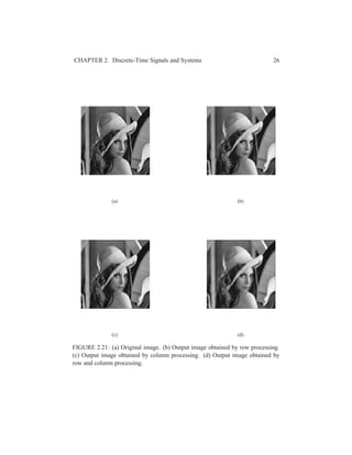
FIGURE 2.20: (a) Original image. (b) Output image processed by 3 × 3 impulse
response h[m, n] given in (2.75). (c) Output image processed by 5 × 5 impulse
response h[m, n] defined in part (c).](https://image.slidesharecdn.com/applied-digital-signal-processing-1st-edition-manolakis-solutions-manual-190422092224/85/Applied-Digital-Signal-Processing-1st-Edition-Manolakis-Solutions-Manual-24-320.jpg)
![CHAPTER 2. Discrete-Time Signals and Systems 25
16. (a) See plots.
(b) Comments: The resulting image is horizontally blurred.
(c) Comments: The resulting image is vertically blurred.
(d) Comments: The resulting image is blurred the same way as the one in
part (c) in Problem 16.
MATLAB script:
% P0216: Filtering 2D image lena.jpg using 1D filter
x = imread(’lena.jpg’);
[nx ny] = size(x);
% Part (a): image show
hfs = figconfg(’0216a’,’small’);
imshow(x,[])
n = -2:2;
h = ones(1,5)/5;
% Part (b): horizontal filtering
yh = zeros(nx,ny);
for ii = 1:ny
temp = conv(h,double(x(ii,:)));
yh(ii,:) = temp(3:end-2);
end
hfs1 = figconfg(’0216b’,’small’);
imshow(yh,[])
% Part (c): vertical filtering
yv = zeros(nx,ny);
for ii = 1:nx
temp = conv(h,double(x(:,ii)));
yv(:,ii) = temp(3:end-2);
end
hfs2 = figconfg(’0216c’,’small’);
imshow(yv,[])
% Part (d): horizontal and vertical filtering
yhv = zeros(nx,ny);
for ii = 1:nx
temp = conv(h,yh(:,ii));
yhv(:,ii) = temp(3:end-2);
end
hfs3 = figconfg(’0216d’,’small’);
imshow(yhv,[])](https://image.slidesharecdn.com/applied-digital-signal-processing-1st-edition-manolakis-solutions-manual-190422092224/85/Applied-Digital-Signal-Processing-1st-Edition-Manolakis-Solutions-Manual-25-320.jpg)
![CHAPTER 2. Discrete-Time Signals and Systems 27
17. (a) Impulse response.
0 10 20 30 40 50 60 70 80 90 100
−0.2
0
0.2
0.4
0.6
n
h[n] Impulse Response h[n]
FIGURE 2.22: Impulse response h[n].
(b) Output using y=filter(b,a,x).
0 10 20 30 40 50 60 70 80 90 100
0
0.5
1
1.5
n
y
1
[n]
Unit Step Response: filter(b,a,x)
FIGURE 2.23: System step output y[n] computed using the function
y=filter(b,a,x).
(c) Output using y=conv(h,x).
(d) Output using y=filter(h,1,x).
MATLAB script:
% P0217: Illustrating the usage of functions ’impz’,’filter,’conv’
close all; clc
n = 0:100;
b = [0.18 0.1 0.3 0.1 0.18];
a = [1 -1.15 1.5 -0.7 0.25];
% Part (a):](https://image.slidesharecdn.com/applied-digital-signal-processing-1st-edition-manolakis-solutions-manual-190422092224/85/Applied-Digital-Signal-Processing-1st-Edition-Manolakis-Solutions-Manual-27-320.jpg)
![CHAPTER 2. Discrete-Time Signals and Systems 28
0 20 40 60 80 100 120 140 160 180 200
−0.5
0
0.5
1
1.5
n
y
2
[n]
Unit Step Response: conv(h,x)
FIGURE 2.24: System step output y[n] computed using the function
y=conv(h,x).
0 10 20 30 40 50 60 70 80 90 100
0
0.5
1
1.5
n
y
3
[n]
Unit Step Response: filter(h,1,x)
FIGURE 2.25: System step output y[n] computed using the function
y=filter(h,1,x).
h = impz(b,a,length(n));
% Part (b):
u = unitstep(n(1),0,n(end));
y1 = filter(b,a,u);
% Part (c):
y2 = conv(h,u);
% Part (d):
y3 = filter(h,1,u);
%Plot
hf = figconfg(’P0217a’,’long’);
stem(n,h,’fill’)
xlabel(’n’,’fontsize’,LFS); ylabel(’h[n]’,’fontsize’,LFS);
title(’Impulse Response h[n]’,’fontsize’,TFS);](https://image.slidesharecdn.com/applied-digital-signal-processing-1st-edition-manolakis-solutions-manual-190422092224/85/Applied-Digital-Signal-Processing-1st-Edition-Manolakis-Solutions-Manual-28-320.jpg)
![CHAPTER 2. Discrete-Time Signals and Systems 29
hf2 = figconfg(’P0217b’,’long’);
stem(n,y1,’fill’)
xlabel(’n’,’fontsize’,LFS); ylabel(’y_1[n]’,’fontsize’,LFS);
title(’Unit Step Response: filter(b,a,x)’,’fontsize’,TFS);
hf3 = figconfg(’P0217c’,’long’);
stem(0:2*n(end),y2,’fill’)
xlabel(’n’,’fontsize’,LFS); ylabel(’y_2[n]’,’fontsize’,LFS);
title(’Unit Step Response: conv(h,x)’,’fontsize’,TFS);
hf4 = figconfg(’P0217d’,’long’);
stem(n,y3,’fill’)
xlabel(’n’,’fontsize’,LFS); ylabel(’y_3[n]’,’fontsize’,LFS);
title(’Unit Step Response: filter(h,1,x)’,’fontsize’,TFS);
18. (a) Block diagrams.
x[n]
y[n]
0.1667 0.1667
z
−1
0.1667
z
−1
0.1667
z
−1
0.1667
z
−1
0.1667
z
−1
FIGURE 2.26: Block diagram representations of the nonrecursive implementation
of M = 5 moving average filter.
(b) MATLAB script:
% P0218: Implement nonrecursive and recursive implementations
% of moving average filter
close all; clc
M = 5;
n = 0:M;
un = unitstep(n(1),0,n(end));
% Nonrecursive implementation:
y_nr = filter(ones(1,M+1)/(M+1),1,un);
% Recursive implementation:
y_re = filter([1 zeros(1,M) -1]/(M+1),[1 -1],un);
hf = figconfg(’P0218’);
subplot(2,1,1)](https://image.slidesharecdn.com/applied-digital-signal-processing-1st-edition-manolakis-solutions-manual-190422092224/85/Applied-Digital-Signal-Processing-1st-Edition-Manolakis-Solutions-Manual-29-320.jpg)
![CHAPTER 2. Discrete-Time Signals and Systems 30
x[n] y[n]
0.1667
0z
−1
0z−1
0z−1
0z−1
0
z−1
−0.1667
z−1
1
FIGURE 2.27: Block diagram representations of the recursive implementation of
M = 5 moving average filter.
stem(n,y_nr,’fill’)
axis([n(1)-1 n(end)+1 min(y_nr)-0.5 max(y_nr)+0.5])
xlabel(’n’,’fontsize’,LFS); ylabel(’y_1[n]’,’fontsize’,LFS);
title(’Nonrecursive Implementation’,’fontsize’,TFS);
subplot(2,1,2)
stem(n,y_re,’fill’)
axis([n(1)-1 n(end)+1 min(y_re)-0.5 max(y_re)+0.5])
xlabel(’n’,’fontsize’,LFS); ylabel(’y_2[n]’,’fontsize’,LFS);
title(’Recursive Implementation’,’fontsize’,TFS);
19. MATLAB script:
% P0219: Generate digital reverberation using audio file ’handel’
close all; clc
load(’handel.mat’)
n = 1:length(y);
a = 0.7; % specify attenuation factor
tau = 50e-3; % Part (a)](https://image.slidesharecdn.com/applied-digital-signal-processing-1st-edition-manolakis-solutions-manual-190422092224/85/Applied-Digital-Signal-Processing-1st-Edition-Manolakis-Solutions-Manual-30-320.jpg)
![CHAPTER 2. Discrete-Time Signals and Systems 31
−1 0 1 2 3 4 5 6
0
0.5
1
1.5
n
y1
[n]
Nonrecursive Implementation
−1 0 1 2 3 4 5 6
0
0.5
1
1.5
n
y2
[n]
Recursive Implementation
FIGURE 2.28: Step response computed by nonrecursive and recursive implemen-
tations.
% tau = 100e-3; % Part (b)
% tau = 500e-3; % Part (c)
D = floor(tau*Fs); % compute delay
yd = filter(1,[1 zeros(1,length(D)-1),-a],y);
sound(yd,Fs)
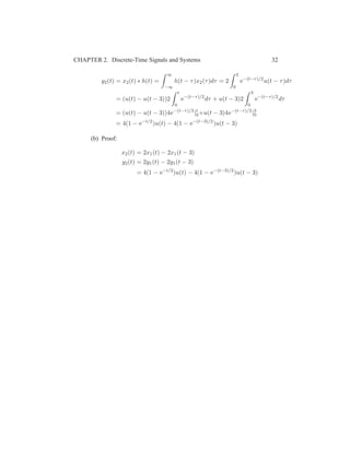
20. (a) Solution:
y1(t) = x1(t) ∗ h(t) =
∞
−∞
h(τ)x1(t − τ)dτ =
∞
−∞
e−τ/2
u(τ)u(t − τ)dτ
= u(t)
t
0
e−τ/2
dτ = u(t)(−2)e−τ/2
|t
0= 2(1 − e−t/2
)u(t)](https://image.slidesharecdn.com/applied-digital-signal-processing-1st-edition-manolakis-solutions-manual-190422092224/85/Applied-Digital-Signal-Processing-1st-Edition-Manolakis-Solutions-Manual-31-320.jpg)
![CHAPTER 2. Discrete-Time Signals and Systems 33
Basic Problems
21. See book companion toolbox for the function.
22. (a) x[n] versus n.
−30 −20 −10 0 10 20 30
−1.5
−1
−0.5
0
0.5
1
1.5
n
x[n]
x[n]
FIGURE 2.29: x[n] versus n.
(b) A down sampled signal y[n] for M = 5.
−30 −20 −10 0 10 20 30
−1.5
−1
−0.5
0
0.5
1
1.5
n
y[n]
Downsampling y[n]= x[nM]
FIGURE 2.30: A down sampled signal y[n] for M = 5.
(c) A down sampled signal y[n] for M = 20.
(d) Comments: The downsampled signal is compressed.
MATLAB script:
% P0222: Illustrate downsampling: y[n] = x[nM]
close all; clc
nx = -30:30;
x = cos(0.1*pi*nx);](https://image.slidesharecdn.com/applied-digital-signal-processing-1st-edition-manolakis-solutions-manual-190422092224/85/Applied-Digital-Signal-Processing-1st-Edition-Manolakis-Solutions-Manual-33-320.jpg)
![CHAPTER 2. Discrete-Time Signals and Systems 34
−30 −20 −10 0 10 20 30
−0.5
0
0.5
1
1.5
n
y[n]
Downsampling y[n]= x[nM]
FIGURE 2.31: A down sampled signal y[n] for M = 20.
% M = 5; % Part (b)
M = 20; % Part (c)
yind = mod(nx,M)==0;
y = x(yind);
ny = nx(yind)/M;
[x y n] = timealign(x,nx,y,ny);
hf = figconfg(’P0222a’,’long’);
stem(n,x,’fill’)
axis([n(1)-1 n(end)+1 min(x)-0.5 max(x)+0.5])
xlabel(’n’,’fontsize’,LFS); ylabel(’x[n]’,’fontsize’,LFS);
title(’x[n]’,’fontsize’,TFS);
hf2 = figconfg(’P0222b’,’long’);
stem(n,y,’fill’)
axis([n(1)-1 n(end)+1 min(y)-0.5 max(y)+0.5])
xlabel(’n’,’fontsize’,LFS); ylabel(’y[n]’,’fontsize’,LFS);
title(’Downsampling y[n]= x[nM]’,’fontsize’,TFS);
23. (a) y[n] = x[−n] (Time-flip)
linear, time-variant, noncausal, and stable
(b) y[n] = log(|x[n]|) (Log-magnitude )
nonlinear, time-invariant, causal, and unstable
(c) y[n] = x[n] − x[n − 1] (First-difference)
linear, time-invariant, causal, and stable
(d) y[n] = round{x[n]} (Quantizer)
nonlinear, time-invariant, causal, and stable](https://image.slidesharecdn.com/applied-digital-signal-processing-1st-edition-manolakis-solutions-manual-190422092224/85/Applied-Digital-Signal-Processing-1st-Edition-Manolakis-Solutions-Manual-34-320.jpg)
![CHAPTER 2. Discrete-Time Signals and Systems 35
24. Comments: The filtered data are smoother and y1[n] is 25 samples delayed
than y2[n].
0 100 200 300 400 500 600
0
200
400
600
800
1000
1200
time index n
DowJonesIndustrialIndex
x[n]
y1
[n]
y2
[n]
FIGURE 2.32: Dow Jones Industrial Average weekly opening value x[n] and its
moving averages.
MATLAB script:
% P0224: Write MATLAB script to compute moving averages
close all; clc
x = load(’djw6576.txt’);
N = length(x);
nx = 0:N-1;
xepd1 = [zeros(50,1);x];
y1 = zeros(N,1);
for ii = 1:N
y1(ii) = sum(xepd1(ii:ii+50))/51;
end
xepd2 = [zeros(25,1);x;zeros(25,1)];](https://image.slidesharecdn.com/applied-digital-signal-processing-1st-edition-manolakis-solutions-manual-190422092224/85/Applied-Digital-Signal-Processing-1st-Edition-Manolakis-Solutions-Manual-35-320.jpg)
![CHAPTER 2. Discrete-Time Signals and Systems 36
y2 = zeros(N,1);
for ii = 1:N
y2(ii) = sum(xepd2(ii:ii+50))/51;
end
% Plot:
hf = figconfg(’P0224’);
plot(nx,x,’.’,nx,y1,’.’,nx,y2,’.’)
xlabel(’time index n’,’fontsize’,LFS)
ylabel(’Dow Jones Industrial Index’,’fontsize’,LFS)
legend(’x[n]’,’y_1[n]’,’y_2[n]’,’fontsize’,LFS,’location’,’best’)
25. (a) Solution:
y[n] = h[n] ∗ x[n] =
∞
m=−∞
h[m]x[n − m]
=
∞
m=−∞
m(u[m] − u[m − M])(u[n − m] − u[n − M − N])
if n ∈[0, M − 1]
y[n] =
n
m=0
m =
n(n + 1)
2
if n ∈[M − 1, N − 1]
y[n] =
M−1
m=0
m =
M(M − 1)
2
if n ∈[N − 1, M + N − 3]
y[n] =
M−1
m=n−(N−1)
m =
M−1
m=0
m −
n−N
m=0
m =
M(M − 1)
2
−
(n − N + 1)(n − N)
2
(b) Comments: The analytical solution can be verified.
MATLAB script:
% P0225: Verify the analytical expression
close all; clc
N = 10; M = 5;
n = 0:N-1;](https://image.slidesharecdn.com/applied-digital-signal-processing-1st-edition-manolakis-solutions-manual-190422092224/85/Applied-Digital-Signal-Processing-1st-Edition-Manolakis-Solutions-Manual-36-320.jpg)
![CHAPTER 2. Discrete-Time Signals and Systems 37
0 5 10 15
0
2
4
6
8
10
n
y[n]
y[n] = h[n]*x[n]
FIGURE 2.33: MATLAB verification of analytical expression for the sequence
y[n] = h[n] ∗ x[n].
x = unitpulse(0,0,N-1,N-1)’;
h = n.*unitpulse(0,0,M-1,N-1)’;
[y ny] = conv0(h,n,x,n);
% Plot:
hf = figconfg(’P0225’,’small’);
stem(ny,y,’fill’)
axis([ny(1)-1,ny(end)+1,min(y)-1,max(y)+1])
xlabel(’n’,’fontsize’,LFS); ylabel(’y[n]’,’fontsize’,LFS);
title(’y[n] = h[n]*x[n]’,’fontsize’,TFS)
26. Solution:
y[n] = x[n] ∗ h[n] =
∞
k=−∞
x[n − k]h[k]
if n ∈[0, N − 1]
y[n] =
n
k=0
ak
=
1 − an+1
1 − a
if n ∈[N − 1, M − 1]
y[n] =
n
k=n−N+1
ak
=
n
k=0
ak
−
n−N
k=0
ak
=
an+1(a−N − 1)
1 − a](https://image.slidesharecdn.com/applied-digital-signal-processing-1st-edition-manolakis-solutions-manual-190422092224/85/Applied-Digital-Signal-Processing-1st-Edition-Manolakis-Solutions-Manual-37-320.jpg)
![CHAPTER 2. Discrete-Time Signals and Systems 38
if n ∈[M − 1, M + N − 2]
y[n] =
M−1
k=n−N+1
ak
=
M−1
k=0
ak
−
n−N
k=0
ak
=
an−N+1 − aM
1 − a
y[n] = 0, otherwise
27. Solution:
y[n] = h[n] ∗ x[n] = an
u[n] ∗ bn
u[n]
=
∞
m=−∞
am
u[m]bn−m
u[n − m] = u[n]
n
m=0
am
bn−m
= u[n]bn
n
m=0
am
b−m
=
bn+1 − an+1
b − a
u[n]
0 5 10 15 20
−0.2
0
0.2
0.4
0.6
0.8
1
n
y[n]
y[n] = h[n]*x[n]
FIGURE 2.34: MATLAB verification of analytical expression for the sequence
y[n] = h[n] ∗ x[n].
MATLAB script:
% P0227: Verify the analytical expression
close all; clc
a = 1/4; b = 1/3;
N = 20;
n = 0:N-1;
x = a.^n;
h = b.^n;
y = conv(h,x);](https://image.slidesharecdn.com/applied-digital-signal-processing-1st-edition-manolakis-solutions-manual-190422092224/85/Applied-Digital-Signal-Processing-1st-Edition-Manolakis-Solutions-Manual-38-320.jpg)
![CHAPTER 2. Discrete-Time Signals and Systems 39
% Plot:
hf = figconfg(’P0227’,’small’);
stem(n,y(1:N),’fill’)
axis([n(1)-1,n(end)+1,min(y)-0.2,max(y)+0.2])
xlabel(’n’,’fontsize’,LFS); ylabel(’y[n]’,’fontsize’,LFS);
title(’y[n] = h[n]*x[n]’,’fontsize’,TFS)
28. (a) Solution:
y[n] = x[n] ∗ h[n] =
∞
m=−∞
(0.9)m
u[m](0.9)n−m
u[n − m]
= u[n]
n
m=0
(0.9)n
= (n + 1)(0.9)n
u[n]
0 10 20 30 40 50 60 70 80 90
0
1
2
3
4
n
y[n]
y[n] = h[n]*x[n] Analytical Expression
FIGURE 2.35: y[n] plot determined analytically.
(b) y[n] computed by conv function.
(c) y[n] computed by filter function.
(d) Comments: (c) comes closer to (a). Because in (b) the tail parts (sam-
ples from n = 50) of both x[n] and h[n] are curtailed, the second part
samples (samples from n = 50) of (b) differ from the ones in (a).
MATLAB script:
% P0228: Verify the analytical expression
close all; clc
a = 0.9;
% Part (a): Analytical Result:](https://image.slidesharecdn.com/applied-digital-signal-processing-1st-edition-manolakis-solutions-manual-190422092224/85/Applied-Digital-Signal-Processing-1st-Edition-Manolakis-Solutions-Manual-39-320.jpg)
![CHAPTER 2. Discrete-Time Signals and Systems 40
0 10 20 30 40 50 60 70 80 90
0
1
2
3
4
n
y
2
[n]
y[n] = h[n]*x[n] Computed by ’conv’
FIGURE 2.36: y[n] plot determined by conv function.
0 10 20 30 40 50 60 70 80 90
0
1
2
3
4
n
y
3
[n]
y[n] = h[n]*x[n] Computed by ’filter’
FIGURE 2.37: y[n] plot determined by filter function.
n = 0:98;
y1 = (n+1).*a.^n;
% Plot:
hf1 = figconfg(’P0228a’,’long’);
stem(n,y1,’fill’)
axis([n(1)-1,n(end)+1,min(y1)-0.2,max(y1)+0.2])
xlabel(’n’,’fontsize’,LFS); ylabel(’y[n]’,’fontsize’,LFS);
title(’y[n] = h[n]*x[n] Analytical Expression’,’fontsize’,TFS)
% Part (b): Using ’conv’
N = 50;
n = 0:N-1;
x = a.^n;
h = a.^n;
y2 = conv(h,x);
ny = 0:length(y2)-1;](https://image.slidesharecdn.com/applied-digital-signal-processing-1st-edition-manolakis-solutions-manual-190422092224/85/Applied-Digital-Signal-Processing-1st-Edition-Manolakis-Solutions-Manual-40-320.jpg)
![CHAPTER 2. Discrete-Time Signals and Systems 41
% Plot:
hf2 = figconfg(’P0228b’,’long’);
stem(ny,y2,’fill’)
axis([ny(1)-1,ny(end)+1,min(y2)-0.2,max(y2)+0.2])
xlabel(’n’,’fontsize’,LFS); ylabel(’y_2[n]’,’fontsize’,LFS);
title(’y[n] = h[n]*x[n] Computed by ’’conv’’’,’fontsize’,TFS)
% Part (c): Using ’filter’
N = 99;
n = 0:N-1;
x = a.^n;
h = a.^n;
y3 = filter(h,1,x);
ny = 0:length(y2)-1;
% Plot:
hf3 = figconfg(’P0228c’,’long’);
stem(ny,y3,’fill’)
axis([ny(1)-1,ny(end)+1,min(y3)-0.2,max(y3)+0.2])
xlabel(’n’,’fontsize’,LFS); ylabel(’y_3[n]’,’fontsize’,LFS);
title(’y[n] = h[n]*x[n] Computed by ’’filter’’’,’fontsize’,TFS)](https://image.slidesharecdn.com/applied-digital-signal-processing-1st-edition-manolakis-solutions-manual-190422092224/85/Applied-Digital-Signal-Processing-1st-Edition-Manolakis-Solutions-Manual-41-320.jpg)
![CHAPTER 2. Discrete-Time Signals and Systems 42
29. MATLAB script:
% P0229: Verify the properites of convolution summarized
% in Table 2.3 on page 54
close all; clc
%% Specify signals:
nx = -15:9;
x = nx*(-1);
nh = 0:9;
h = 0.5.^nh;
nh1 = 0:20;
h1 = cos(0.05*pi*nh1);
nh2 = -3:5;
h2 = [2 0 0 0 2 0 0 0 -3];
[d nd] = delta(0,0,0); % unit impulse
n0 = 3;
[dd ndd] = delta(n0,n0,n0); % unit delay
%% Verify Identity Property:
y = conv(x,d);
% Plot:
hf1 = figconfg(’P0229a’);
subplot(2,1,1)
stem(nx,x,’fill’)
axis([nx(1)-1,nx(end)+1,min(x)-1,max(x)+1])
xlabel(’n’,’fontsize’,LFS); ylabel(’x[n]’,’fontsize’,LFS)
title(’x[n]’,’fontsize’,TFS)
subplot(2,1,2)
stem(nx,y,’fill’)
axis([nx(1)-1,nx(end)+1,min(y)-1,max(y)+1])
xlabel(’n’,’fontsize’,LFS); ylabel(’y[n]’,’fontsize’,LFS);
title(’y[n] = x[n]times delta[n]’,’fontsize’,TFS)
%% Verify Delay Property:
[y1 ny1] = shift(x,nx,-n0);
y2 = conv(x,dd);
ny2 = nx + n0;
% Plot:
hf2 = figconfg(’P0229b’);
subplot(2,1,1)
stem(ny1,y1,’fill’)
axis([ny1(1)-1,ny1(end)+1,min(y1)-1,max(y1)+1])](https://image.slidesharecdn.com/applied-digital-signal-processing-1st-edition-manolakis-solutions-manual-190422092224/85/Applied-Digital-Signal-Processing-1st-Edition-Manolakis-Solutions-Manual-42-320.jpg)
![CHAPTER 2. Discrete-Time Signals and Systems 43
xlabel(’n’,’fontsize’,LFS);
title(’x[n-n_0]’,’fontsize’,TFS)
subplot(2,1,2)
stem(ny2,y2,’fill’)
axis([ny2(1)-1,ny2(end)+1,min(y2)-1,max(y2)+1])
xlabel(’n’,’fontsize’,LFS)
title(’x[n]times delta[n-n_0]’,’fontsize’,TFS)
%% Verify Commutative Property:
y1 = conv(x,h);
ny1 = nx(1)+nh(1):nx(end)+nh(end);
y2 = conv(h,x);
ny2 = nx(1)+nh(1):nx(end)+nh(end);
% Plot:
hf3 = figconfg(’P0229c’);
subplot(2,1,1)
stem(ny1,y1,’fill’)
axis([ny1(1)-1,ny1(end)+1,min(y1)-1,max(y1)+1])
xlabel(’n’,’fontsize’,LFS)
title(’x[n]times h[n]’,’fontsize’,TFS)
subplot(2,1,2)
stem(ny2,y2,’fill’)
axis([ny2(1)-1,ny2(end)+1,min(y2)-1,max(y2)+1])
xlabel(’n’,’fontsize’,LFS)
title(’h[n]times x[n]’,’fontsize’,TFS)
%% Verify Associative Property:
[y1 ny1] = conv0(x,nx,h1,nh1);
[y1 ny1] = conv0(y1,ny1,h2,nh2);
[y2 ny2] = conv0(h1,nh1,h2,nh2);
[y2 ny2] = conv0(x,nx,y2,ny2);
% Plot:
hf4 = figconfg(’P0229d’);
subplot(2,1,1)
stem(ny1,y1,’fill’)
axis([ny1(1)-1,ny1(end)+1,min(y1)-1,max(y1)+1])
xlabel(’n’,’fontsize’,LFS)
title(’(x[n]times h_1[n])times h_2[n]’,’fontsize’,TFS)
subplot(2,1,2)
stem(ny2,y2,’fill’)
axis([ny2(1)-1,ny2(end)+1,min(y2)-1,max(y2)+1])
xlabel(’n’,’fontsize’,LFS)](https://image.slidesharecdn.com/applied-digital-signal-processing-1st-edition-manolakis-solutions-manual-190422092224/85/Applied-Digital-Signal-Processing-1st-Edition-Manolakis-Solutions-Manual-43-320.jpg)
![CHAPTER 2. Discrete-Time Signals and Systems 44
title(’x[n]times (h_1[n]times h_2[n])’,’fontsize’,TFS)
%% Verify Distributive Property:
[hh1 hh2 nh12] = timealign(h1,nh1,h2,nh2);
[y1 ny1] = conv0(x,nx,hh1+hh2,nh12);
[y2a ny2a] = conv0(x,nx,h1,nh1);
[y2b ny2b] = conv0(x,nx,h2,nh2);
[y2a y2b ny2] = timealign(y2a,ny2a,y2b,ny2b);
y2 = y2a + y2b;
% Plot:
hf5 = figconfg(’P0229e’);
subplot(2,1,1)
stem(ny1,y1,’fill’)
axis([ny1(1)-1,ny1(end)+1,min(y1)-1,max(y1)+1])
xlabel(’n’,’fontsize’,LFS)
title(’x[n]times (h_1[n]+h_2[n])’,’fontsize’,TFS)
subplot(2,1,2)
stem(ny2,y2,’fill’)
axis([ny2(1)-1,ny2(end)+1,min(y2)-1,max(y2)+1])
xlabel(’n’,’fontsize’,LFS)
title(’x[n]times h_1[n]+x[n]times h_2[n]’,’fontsize’,TFS)](https://image.slidesharecdn.com/applied-digital-signal-processing-1st-edition-manolakis-solutions-manual-190422092224/85/Applied-Digital-Signal-Processing-1st-Edition-Manolakis-Solutions-Manual-44-320.jpg)
![CHAPTER 2. Discrete-Time Signals and Systems 45
−15 −10 −5 0 5 10
−10
−5
0
5
10
15
n
x[n]
x[n]
−15 −10 −5 0 5 10
−10
−5
0
5
10
15
n
y[n]
y[n] = x[n]× δ[n]
FIGURE 2.38: Verify identity property.
−10 −5 0 5 10
−10
−5
0
5
10
15
n
x[n−n
0
]
−10 −5 0 5 10
−10
−5
0
5
10
15
n
x[n]× δ[n−n
0
]
FIGURE 2.39: Verify delay property.](https://image.slidesharecdn.com/applied-digital-signal-processing-1st-edition-manolakis-solutions-manual-190422092224/85/Applied-Digital-Signal-Processing-1st-Edition-Manolakis-Solutions-Manual-45-320.jpg)
![CHAPTER 2. Discrete-Time Signals and Systems 46
−15 −10 −5 0 5 10 15
−10
0
10
20
n
x[n]× h[n]
−15 −10 −5 0 5 10 15
−10
0
10
20
n
h[n]× x[n]
FIGURE 2.40: Verify commutative property.
−15 −10 −5 0 5 10 15 20 25 30 35
−300
−200
−100
0
100
200
n
(x[n]× h
1
[n])× h
2
[n]
−15 −10 −5 0 5 10 15 20 25 30 35
−300
−200
−100
0
100
200
n
x[n]× (h
1
[n]× h
2
[n])
FIGURE 2.41: Verify associative property.](https://image.slidesharecdn.com/applied-digital-signal-processing-1st-edition-manolakis-solutions-manual-190422092224/85/Applied-Digital-Signal-Processing-1st-Edition-Manolakis-Solutions-Manual-46-320.jpg)
![CHAPTER 2. Discrete-Time Signals and Systems 47
−15 −10 −5 0 5 10 15 20 25 30
−100
−50
0
50
100
n
x[n]× (h
1
[n]+h
2
[n])
−15 −10 −5 0 5 10 15 20 25 30
−100
−50
0
50
100
n
x[n]× h1
[n]+x[n]× h2
[n]
FIGURE 2.42: Verify distributive property.
30. MATLAB script:
function [y,L1,L2] = convol(h,M1,M2,x,N1,N2)
% P0230: Compute the convolution of two arbitrarily positioned finite
% length sequences using the procedure illustrated in Figure 2.16
L1 = M1+N1; L2 = M2+N2;
ny = L1:L2;
y = zeros(1,length(ny));
nx = N1:N2;
[hf nhf] = fold(h,M1:M2);
for ii = 1:length(ny)
[hfs nhfs] = shift(hf,nhf,-ny(ii));
[y1 y2 ny] = timealign(hfs,nhfs,x,nx);
y(ii) = sum(y1.*y2);
end](https://image.slidesharecdn.com/applied-digital-signal-processing-1st-edition-manolakis-solutions-manual-190422092224/85/Applied-Digital-Signal-Processing-1st-Edition-Manolakis-Solutions-Manual-47-320.jpg)
![CHAPTER 2. Discrete-Time Signals and Systems 48
31. (a) See below.
0 10 20 30 40 50 60 70 80 90 100
0
1
2
3
4
5
x 10
20
n
y[n] LCCDE: y[n] = y[n−1] + y[n−2] + x[n], y[−1] = y[−2] = 0
FIGURE 2.43: System impulse response for 0 ≤ n ≤ 100, using function filter.
(b) Comments: The system is unstable.
(c) Comments: h[n] is 1 sample left moved Fibonacci sequence.
MATLAB script:
% P0231: Use function ’filter’ to realize LCCDE resting
% at zero initial condition
close all; clc
% Part (a):
n = 0:100;
x = delta(n(1),0,n(end));
y = filter(1,[1 -1 -1],x);
% Plot:
hf = figconfg(’P0231’);
stem(n,y,’fill’)
axis([n(1)-1,n(end)+1,min(y)-1,max(y)+1])
xlabel(’n’,’fontsize’,LFS); ylabel(’y[n]’,’fontsize’,LFS)
title(’LCCDE: y[n] = y[n-1] + y[n-2] + x[n], y[-1] = y[-2] = 0’...
,’fontsize’,TFS)](https://image.slidesharecdn.com/applied-digital-signal-processing-1st-edition-manolakis-solutions-manual-190422092224/85/Applied-Digital-Signal-Processing-1st-Edition-Manolakis-Solutions-Manual-48-320.jpg)
![CHAPTER 2. Discrete-Time Signals and Systems 49
32. MATLAB script:
% P0232: Use function ’filter’ to study the impulse response and
% step response of a system specified by LCCDE
close all; clc
N = 60;
n = 0:N-1;
b = [0.18 0.1 0.3 0.1 0.18];
a = [1 -1.15 1.5 -0.7 0.25];
[d nd] = delta(n(1),0,n(end));
[u nu] = unitstep(n(1),0,n(end));
y1 = filter(b,a,d);
y2 = filter(b,a,u);
% Plot:
hf = figconfg(’P0232’);
subplot(2,1,1)
stem(n,y1,’fill’)
axis([n(1)-1,n(end)+1,min(y1)-0.2,max(y1)+0.2])
xlabel(’n’,’fontsize’,LFS)
title(’Impulse Response’,’fontsize’,TFS);
subplot(2,1,2)
stem(n,y2,’fill’)
axis([n(1)-1,n(end)+1,min(y2)-0.5,max(y2)+0.5])
xlabel(’n’,’fontsize’,LFS)
title(’Step Response’,’fontsize’,TFS)
33. MATLAB script:
% P0233: Realize a first-order digital differentiator given by
% y[n] = x[n] - x[n-1]
close all; clc
% Part (a):
n = -10:19;
x = 10*ones(1,length(n));
% % Part (b):
% nx1 = 0:9;
% x1 = nx1;
% nx2 = 10:19;
% x2 = 20-nx2;](https://image.slidesharecdn.com/applied-digital-signal-processing-1st-edition-manolakis-solutions-manual-190422092224/85/Applied-Digital-Signal-Processing-1st-Edition-Manolakis-Solutions-Manual-49-320.jpg)
![CHAPTER 2. Discrete-Time Signals and Systems 50
0 10 20 30 40 50 60
−0.2
0
0.2
0.4
n
Impulse Response
0 10 20 30 40 50 60
0
0.5
1
1.5
n
Step Response
FIGURE 2.44: System impulse response and step response for first 60 samples
using function filter.
% [x1 x2 n] = timealign(x1,nx1,x2,nx2);
% x = x1 + x2;
% % Part (c):
% n = 0:39;
% x = cos(0.2*pi*n-pi/2);
% Differentiator:
y = filter([1,-1],1,x);
% Plot:
hf = figconfg(’P0233’);
subplot(2,1,1)
stem(n,x,’fill’)
axis([n(1)-1,n(end)+1,min(x)-1,max(x)+1])
xlabel(’n’,’fontsize’,LFS)
title(’Input Signal x[n]’,’fontsize’,TFS)
subplot(2,1,2)
stem(n,y,’fill’)](https://image.slidesharecdn.com/applied-digital-signal-processing-1st-edition-manolakis-solutions-manual-190422092224/85/Applied-Digital-Signal-Processing-1st-Edition-Manolakis-Solutions-Manual-50-320.jpg)
![CHAPTER 2. Discrete-Time Signals and Systems 51
axis([n(1)-1,n(end)+1,min(y)-1,max(y)+1])
xlabel(’n’,’fontsize’,LFS)
title(’Response y[n] = x[n] - x[n-1]’,’fontsize’,LFS)
−10 −5 0 5 10 15 20
9
9.5
10
10.5
11
n
Input Signal x[n]
−10 −5 0 5 10 15 20
0
2
4
6
8
10
n
Response y[n] = x[n] − x[n−1]
FIGURE 2.45: Differentiator output if input is x[n] = 10{u[n + 10] − u[n − 20]}.
34. MATLAB script:
% P0234: Use function ’filter’ to study the impulse response
% and step response of a system specified by LCCDE
close all; clc
N = 100;
n = 0:N-1;
b = 1;
a = [1 -0.9 0.81];
% a = [1 0.9 -0.81];
[d nd] = delta(n(1),0,n(end));
[u nu] = unitstep(n(1),0,n(end));
y1 = filter(b,a,d);
y2 = filter(b,a,u);
% Plot:](https://image.slidesharecdn.com/applied-digital-signal-processing-1st-edition-manolakis-solutions-manual-190422092224/85/Applied-Digital-Signal-Processing-1st-Edition-Manolakis-Solutions-Manual-51-320.jpg)
![CHAPTER 2. Discrete-Time Signals and Systems 52
0 2 4 6 8 10 12 14 16 18 20
0
2
4
6
8
10
n
Input Signal x[n]
0 2 4 6 8 10 12 14 16 18 20
−2
−1
0
1
2
n
Response y[n] = x[n] − x[n−1]
FIGURE 2.46: Differentiator output if input is x[n] = n{u[n]−u[n−10]}+(20−
n){u[n − 10] − u[n − 20]}.
hf = figconfg(’P0234a’,’long’);
stem(n,y1,’fill’)
axis([n(1)-1,n(end)+1,min(y1)-1,max(y1)+1])
xlabel(’n’,’fontsize’,LFS)
title(’Impulse Response’,’fontsize’,TFS)
hf2 = figconfg(’P0234b’,’long’);
stem(n,y2,’fill’)
axis([n(1)-1,n(end)+1,min(y2)-1,max(y2)+1])
xlabel(’n’,’fontsize’,LFS)
title(’Step Response’,’fontsize’,TFS)
35. (a) y(t) = x(t − 1) + x(2 − t)
linear, time-variant, noncausal, and stable
(b) y(t) = dx(t)/dt
linear, time-invariant, causal, and unstable
(c) y(t) =
3t
−∞ x(τ)dτ
linear, time-variant, noncausal, and unstable](https://image.slidesharecdn.com/applied-digital-signal-processing-1st-edition-manolakis-solutions-manual-190422092224/85/Applied-Digital-Signal-Processing-1st-Edition-Manolakis-Solutions-Manual-52-320.jpg)
![CHAPTER 2. Discrete-Time Signals and Systems 53
0 5 10 15 20 25 30 35 40
−1
0
1
n
Input Signal x[n]
0 5 10 15 20 25 30 35 40
−1
0
1
n
Response y[n] = x[n] − x[n−1]
FIGURE 2.47: Differentiator output if input is x[n] = cos(0.2πn − π/2){u[n] −
u[n − 40]}.
(d) y(t) = 2x(t) + 5
nonlinear, time-invariant, causal, and stable
36. (a) Solution:
y(t) = h(t) ∗ x(t) =
∞
−∞
x(τ)h(t − τ)dτ
if t ∈[−1, 1]
y(t) =
1+t
0
τ/3dτ =
(1 + t)2
6
if t ∈[1, 2]
y(t) =
1+t
−1+t
τ/3dτ =
2t
3
if t ∈[2, 4]
y(t) =
3
−1+t
τ/3dτ =
−t2 + 2t + 8
6
y(t) = 0 otherwise](https://image.slidesharecdn.com/applied-digital-signal-processing-1st-edition-manolakis-solutions-manual-190422092224/85/Applied-Digital-Signal-Processing-1st-Edition-Manolakis-Solutions-Manual-53-320.jpg)
![CHAPTER 2. Discrete-Time Signals and Systems 54
0 10 20 30 40 50 60 70 80 90 100
−1.5
−1
−0.5
0
0.5
1
1.5
2
n
Impulse Response
FIGURE 2.48: System impulse response.
0 10 20 30 40 50 60 70 80 90 100
0
0.5
1
1.5
2
2.5
n
Step Response
FIGURE 2.49: System step response.
(b) Proof:
y(t) = h(t) ∗ x(t) =
∞
−∞
h(τ)x(t − τ)dτ
=
∞
k=−∞
T
2
− T
2
h(kT + τ)x(t − kT − τ)dτ
≈
∞
k=−∞
[h(kT)x(t − kT)T]
= T
∞
k=−∞
h[k]x[n − k] = ˆy(t)
(c) Comments: When T = 0.01, the error becomes negligible.
MATLAB script:](https://image.slidesharecdn.com/applied-digital-signal-processing-1st-edition-manolakis-solutions-manual-190422092224/85/Applied-Digital-Signal-Processing-1st-Edition-Manolakis-Solutions-Manual-54-320.jpg)
![CHAPTER 2. Discrete-Time Signals and Systems 55
−1 −0.5 0 0.5 1 1.5 2 2.5 3 3.5 4
0
0.5
1
1.5
MSE = 0.003512
t (∆ T = 0.1)
yhat[n]
y[n]
FIGURE 2.50: Plot of sequences ˆy(nT) and y(nT) for T = 0.1.
% P0236: Compute and plot continuous-time convolution
% using discrete approximation
close all; clc
dT = 0.1;
% % dT = 0.01;
n = -1/dT:4/dT;
t = n*dT;
h = zeros(1,length(n));
ind = (t >= -1 & t <=1);
h(ind) = 1;
x = zeros(1,length(n));
ind = (t >= 0 & t <=3);
x(ind) = t(ind)/3;
% Theoretical continuous y(t):
y = zeros(1,length(n));
ind = (t >= -1 & t <= 1);
y(ind) = (t(ind).^2+2*t(ind)+1)/6;
ind = (t >=1 & t <= 2);
y(ind) = 2*t(ind)/3;
ind = (t >=2 & t <= 4);](https://image.slidesharecdn.com/applied-digital-signal-processing-1st-edition-manolakis-solutions-manual-190422092224/85/Applied-Digital-Signal-Processing-1st-Edition-Manolakis-Solutions-Manual-55-320.jpg)
![CHAPTER 2. Discrete-Time Signals and Systems 56
−1 −0.5 0 0.5 1 1.5 2 2.5 3 3.5 4
0
0.2
0.4
0.6
0.8
1
1.2
1.4
MSE = 3.4845e−05
t (∆ T = 0.01)
yhat[n]
y[n]
FIGURE 2.51: Plot of sequences ˆy(nT) and y(nT) for T = 0.01.
y(ind) = (-t(ind).^2+2*t(ind)+8)/6;
% Approximated y(t):
[yhat nyhat] = conv0(h,n,x,n);
tyhat = dT*nyhat;
yhat = dT*yhat;
ind = (tyhat <-1 | tyhat>4);
yhat(ind) = [];
% Compute mean square error:
mse = mean((y-yhat).^2);
% Plot:
hf1 = figconfg(’P0236’);
plot(t,yhat,’.’,t,y,’-.’)
TB = [’MSE = ’,num2str(mse)];
title(TB,’fontsize’,TFS)
LB = [’t (Delta T = ’,num2str(dT),’)’];
xlabel(LB,’fontsize’,LFS);
legend(’yhat[n]’,’y[n]’,’location’,’best’)](https://image.slidesharecdn.com/applied-digital-signal-processing-1st-edition-manolakis-solutions-manual-190422092224/85/Applied-Digital-Signal-Processing-1st-Edition-Manolakis-Solutions-Manual-56-320.jpg)
![CHAPTER 2. Discrete-Time Signals and Systems 57
Assessment Problems
37. Comments: y1[n] represents the correct x[−n − 4] signal.
−10 −9 −8 −7 −6 −5 −4 −3 −2 −1 0 1 2 3 4 5
−1
0
1
2
3
4
5
6
n
y
1
[n]
First Folding Then Shifting
FIGURE 2.52: y1[n] obtained by first folding and then shifting.
−10 −9 −8 −7 −6 −5 −4 −3 −2 −1 0 1 2 3 4 5
−1
0
1
2
3
4
5
6
n
y
2
[n]
First Shifting Then Folding
FIGURE 2.53: y2[n] obtained by first shifting and then folding.
MATLAB script:
% P0237: Exercise the manipulations of folding and shifting signals
close all; clc
nx = 0:5;
x = 0:5;
n0 = 4;
% Part (a): First folding, then shifting
[y1 ny1] = fold(x,nx);
[y1 ny1] = shift(y1,ny1,n0);](https://image.slidesharecdn.com/applied-digital-signal-processing-1st-edition-manolakis-solutions-manual-190422092224/85/Applied-Digital-Signal-Processing-1st-Edition-Manolakis-Solutions-Manual-57-320.jpg)
![CHAPTER 2. Discrete-Time Signals and Systems 58
% Part (b): First shifting, then folding
[y2 ny2] = shift(x,nx,n0);
[y2 ny2] = fold(y2,ny2);
% Plot:
hf = figconfg(’P0237a’,’small’);
stem(ny1,y1,’fill’)
xlim([min([ny1(1),ny2(1)])-1,max([ny1(end),ny2(end)])+1])
ylim([min(y1)-1,max(y1)+1])
xlabel(’n’,’fontsize’,LFS); ylabel(’y_1[n]’,’fontsize’,LFS)
title(’First Folding Then Shifting’,’fontsize’,TFS)
set(gca,’Xtick’,min([ny1(1),ny2(1)])-1:max([ny1(end),ny2(end)])+1)
hf2 = figconfg(’P0237b’,’small’);
stem(ny2,y2,’fill’)
xlim([min([ny1(1),ny2(1)])-1,max([ny1(end),ny2(end)])+1])
ylim([min(y2)-1,max(y2)+1])
xlabel(’n’,’fontsize’,LFS); ylabel(’y_2[n]’,’fontsize’,LFS)
title(’First Shifting Then Folding’,’fontsize’,TFS)
set(gca,’Xtick’,min([ny1(1),ny2(1)])-1:max([ny1(end),ny2(end)])+1)
38. MATLAB script:
% P0238: Generate and plot signals using function ’stem’
close all; clc
%% Part (a):
[x1a nx1a] = delta(-1,-1,-1);
x1a = 5*x1a;
nx1b = -5:3;
x1b = nx1b.^2;
nx1c = 4:7;
x1c = 10*0.5.^nx1c;
[x1a x1b nx1] = timealign(x1a,nx1a,x1b,nx1b);
x1 = x1a + x1b;
[x1 x1c nx1] = timealign(x1,nx1,x1c,nx1c);
x1 = x1 + x1c;
% Plot:
hf1 = figconfg(’P0238a’,’small’);
stem(nx1,x1,’fill’)
axis([min(nx1)-1,max(nx1)+1,min(x1)-1,max(x1)+1])
xlabel(’n’,’fontsize’,LFS); ylabel(’x_1[n]’,’fontsize’,LFS)
title(’x_1[n]’,’fontsize’,TFS)](https://image.slidesharecdn.com/applied-digital-signal-processing-1st-edition-manolakis-solutions-manual-190422092224/85/Applied-Digital-Signal-Processing-1st-Edition-Manolakis-Solutions-Manual-58-320.jpg)
![CHAPTER 2. Discrete-Time Signals and Systems 59
set(gca,’Xtick’,nx1(1)-1:nx1(end)+1)
%% Part (b):
nx2 = 0:20;
x2 = 0.8.^nx2.*cos(0.2*pi*nx2+pi/4);
% Plot:
hf2 = figconfg(’P0238b’,’small’);
stem(nx2,x2,’fill’)
axis([min(nx2)-1,max(nx2)+1,min(x2)-0.2,max(x2)+0.2])
xlabel(’n’,’fontsize’,LFS); ylabel(’x_2[n]’,’fontsize’,LFS)
title(’x_2[n]’,’fontsize’,TFS)
%% Part (c):
nx3 = 0:20;
x3 = zeros(1,length(nx3));
for ii = 0:4
[d1 nd1] = delta(nx3(1),ii,nx3(end));
[d2 nd2] = delta(nx3(1),2*ii,nx3(end));
x3 = x3 + (ii+1)*(d1-d2)’;
end
% Plot:
hf3 = figconfg(’P0238c’,’small’);
stem(nx3,x3,’fill’)
axis([min(nx3)-1,max(nx3)+1,min(x3)-1,max(x3)+1])
xlabel(’n’,’fontsize’,LFS); ylabel(’x_3[n]’,’fontsize’,LFS)
title(’x_3[n]’,’fontsize’,TFS)
−6 −5 −4 −3 −2 −1 0 1 2 3 4 5 6 7 8
0
5
10
15
20
25
n
x
1
[n]
x
1
[n]
FIGURE 2.54: x1[n] = 5δ[n + 1] + n2(u[n + 5] − u[n − 4]) + 10(0.5)n(u[n −
4] − u[n − 8]).](https://image.slidesharecdn.com/applied-digital-signal-processing-1st-edition-manolakis-solutions-manual-190422092224/85/Applied-Digital-Signal-Processing-1st-Edition-Manolakis-Solutions-Manual-59-320.jpg)
![CHAPTER 2. Discrete-Time Signals and Systems 60
0 5 10 15 20
−0.5
0
0.5
n
x2
[n]
x
2
[n]
FIGURE 2.55: x2[n] = (0.8)n cos(0.2πn + π/4), 0 ≤ n ≤ 20.
0 5 10 15 20
−6
−4
−2
0
2
4
n
x
3
[n]
x
3
[n]
FIGURE 2.56: x3[n] = 4
m=0(m + 1){δ[n − m] − δ[n − 2m]}, 0 ≤ n ≤ 20.
39. MATLAB script:
% P0239: Generate and plot signals using function ’stem’
close all; clc
nx = -5:14;
x = nx;
x(x<0) = 0;
x(x>10) = 0;
% Part (a):
[x1 nx1] = shift(x,nx,-4);
x1 = 2*x1;
% Part (b):
[x2 nx2] = shift(x,nx,-5);](https://image.slidesharecdn.com/applied-digital-signal-processing-1st-edition-manolakis-solutions-manual-190422092224/85/Applied-Digital-Signal-Processing-1st-Edition-Manolakis-Solutions-Manual-60-320.jpg)
![CHAPTER 2. Discrete-Time Signals and Systems 61
x2 = 3*x2;
% Part (c):
[x3 nx3] = shift(x,nx,3);
[x3 nx3] = fold(x3,nx3);
% Plot:
hf = figconfg(’P0239’);
xlimit = [min([nx(1) nx1(1) nx2(1) nx3(1)])-1,...
max([nx(end) nx1(end) nx2(end) nx3(end)])+1];
subplot(2,2,1)
stem(nx,x,’fill’)
xlim(xlimit); ylim([min(x)-1,max(x)+1])
xlabel(’n’,’fontsize’,LFS); title(’x[n]’,’fontsize’,LFS)
subplot(2,2,2)
stem(nx1,x1,’fill’)
xlim(xlimit); ylim([min(x1)-1,max(x1)+1])
xlabel(’n’,’fontsize’,LFS); title(’2x[n-4]’,’fontsize’,TFS)
subplot(2,2,3)
stem(nx2,x2,’fill’)
xlim(xlimit)
ylim([min(x2)-1,max(x2)+1])
xlabel(’n’);
title(’3x[n-5]’)
subplot(2,2,4)
stem(nx3,x3,’fill’)
xlim(xlimit); ylim([min(x3)-1,max(x3)+1])
xlabel(’n’,’fontsize’,LFS);
title(’x[3-n]’,’fontsize’,TFS)
40.
T{a1x1[n] + a2x2[n]} = 10(a1x1[n] + a2x2[n]) cos(0.25πn + θ)
= a1y1[n] + a2y2[n]
The system is linear.
T{x[n − n0]} = 10x[n − n0] cos(0.25πn + θ)
= y[n − n0] = 10x[n − n0] cos(0.25π(n − n0) + θ)
The system is time-variant.
h[n] = 10δ[n] cos(0.25πn + θ)
The system is causal and stable.](https://image.slidesharecdn.com/applied-digital-signal-processing-1st-edition-manolakis-solutions-manual-190422092224/85/Applied-Digital-Signal-Processing-1st-Edition-Manolakis-Solutions-Manual-61-320.jpg)
![CHAPTER 2. Discrete-Time Signals and Systems 62
−10 −5 0 5 10 15 20
0
2
4
6
8
10
n
x[n]
−10 −5 0 5 10 15 20
0
5
10
15
20
n
2x[n−4]
−10 −5 0 5 10 15 20
0
10
20
30
n
3x[n−5]
−10 −5 0 5 10 15 20
0
2
4
6
8
10
n
x[3−n]
FIGURE 2.57: x[n], 2x[n − 4], 3x[n − 5], and x[3 − n].
41. Comments: The system is unstable.
MATLAB script:
% P0241: Compute and plot the output of the discrete-time system
% y[n] = 5y[n-1]+x[n], y[-1]=0
close all; clc
n = 0:1e3;
x = ones(1,length(n));
y = filter(1,[1 -5],x);
% Plot:
hf = figconfg(’P0241’,’small’);
stem(n,y,’fill’)
axis([n(1)-1 n(end)+1 min(y)-1 max(y)+1])
xlabel(’n’,’fontsize’,LFS);
title(’y[n] = 5y[n-1]+x[n], y[-1]=0’,’fontsize’,TFS)
42. MATLAB script:](https://image.slidesharecdn.com/applied-digital-signal-processing-1st-edition-manolakis-solutions-manual-190422092224/85/Applied-Digital-Signal-Processing-1st-Edition-Manolakis-Solutions-Manual-62-320.jpg)
![CHAPTER 2. Discrete-Time Signals and Systems 63
0 200 400 600 800 1000
0
1
2
3
4
x 10
307
n
y[n] = 5y[n−1]+x[n], y[−1]=0
FIGURE 2.58: Step response of system y[n] = 5y[n − 1] + x[n], y[−1] = 0.
% P0242: Compute the outputs of a LTI system defined by
% ’y=angosto(x)’ for different inputs
close all; clc
n = 0:100;
[d nd] = delta(n(1),0,n(end));
h = agnosto(d);
x1 = ones(1,length(n));
x2 = (1/2).^n;
x3 = cos(2*pi*n/20);
y1 = conv(h,x1);
y2 = conv(h,x2);
y3 = conv(h,x3);
% Reference:
yr1 = agnosto(x1);
yr2 = agnosto(x2);
yr3 = agnosto(x3);
% Plot:
hf1 = figconfg(’P0242a’);
subplot(2,1,1)
stem(n,y1(1:length(n)),’fill’)
axis([n(1)-1 n(end)+1 min(y1(1:length(n)))-1 max(y1(1:length(n)))+1])
xlabel(’n’,’fontsize’,LFS);
title(’y_1[n] Computed by Impulse Response h[n]’,’fontsize’,TFS)
subplot(2,1,2)
stem(n,yr1,’fill’)
axis([n(1)-1 n(end)+1 min(yr1)-1 max(yr1)+1])](https://image.slidesharecdn.com/applied-digital-signal-processing-1st-edition-manolakis-solutions-manual-190422092224/85/Applied-Digital-Signal-Processing-1st-Edition-Manolakis-Solutions-Manual-63-320.jpg)
![CHAPTER 2. Discrete-Time Signals and Systems 64
xlabel(’n’,’fontsize’,LFS);
title(’y_1[n] Computed by Function ’’agnosto’’ Directly’,’fontsize’,TFS)
% Plot:
hf2 = figconfg(’P0242b’);
subplot(2,1,1)
stem(n,y2(1:length(n)),’fill’)
axis([n(1)-1 n(end)+1 min(y2(1:length(n)))-1 max(y2(1:length(n)))+1])
xlabel(’n’,’fontsize’,LFS);
title(’y_2[n] Computed by Impulse Response h[n]’,’fontsize’,TFS)
subplot(2,1,2)
stem(n,yr2,’fill’)
axis([n(1)-1 n(end)+1 min(yr2)-1 max(yr2)+1])
xlabel(’n’,’fontsize’,LFS);
title(’y_2[n] Computed by Function ’’agnosto’’ Directly’,’fontsize’,TFS)
% Plot:
hf3 = figconfg(’P0242c’);
subplot(2,1,1)
stem(n,y3(1:length(n)),’fill’)
axis([n(1)-1 n(end)+1 min(y3(1:length(n)))-1 max(y3(1:length(n)))+1])
xlabel(’n’,’fontsize’,LFS);
title(’y_3[n] Computed by Impulse Response h[n]’,’fontsize’,LFS)
subplot(2,1,2)
stem(n,yr3,’fill’)
axis([n(1)-1 n(end)+1 min(yr3)-1 max(yr3)+1])
xlabel(’n’,’fontsize’,LFS);
title(’y_3[n] Computed by Function ’’agnosto’’ Directly’,’fontsize’,LFS)](https://image.slidesharecdn.com/applied-digital-signal-processing-1st-edition-manolakis-solutions-manual-190422092224/85/Applied-Digital-Signal-Processing-1st-Edition-Manolakis-Solutions-Manual-64-320.jpg)
![CHAPTER 2. Discrete-Time Signals and Systems 65
0 10 20 30 40 50 60 70 80 90 100
0
1
2
3
4
n
y
1
[n] Computed by Impulse Response h[n]
0 10 20 30 40 50 60 70 80 90 100
0
1
2
3
4
n
y1
[n] Computed by Function ’agnosto’ Directly
FIGURE 2.59: System response y1[n] of input x1[n] = u[n].
0 10 20 30 40 50 60 70 80 90 100
−2
−1
0
1
2
n
y2
[n] Computed by Impulse Response h[n]
0 10 20 30 40 50 60 70 80 90 100
−2
−1
0
1
2
n
y
2
[n] Computed by Function ’agnosto’ Directly
FIGURE 2.60: System response y2[n] of input x2[n] = (1/2)n.](https://image.slidesharecdn.com/applied-digital-signal-processing-1st-edition-manolakis-solutions-manual-190422092224/85/Applied-Digital-Signal-Processing-1st-Edition-Manolakis-Solutions-Manual-65-320.jpg)
![CHAPTER 2. Discrete-Time Signals and Systems 66
0 10 20 30 40 50 60 70 80 90 100
−2
0
2
n
y3
[n] Computed by Impulse Response h[n]
0 10 20 30 40 50 60 70 80 90 100
−2
0
2
n
y
3
[n] Computed by Function ’agnosto’ Directly
FIGURE 2.61: System response y3[n] of input x3[n] = cos(2πn/20).
43. (a) Proof:
Ay =
n
y[n] =
n
∞
k=−∞
x[k]h[n − k] =
∞
k=−∞
x[k]
n
h[n − k]
=
∞
k=−∞
x[k]
n
h[n] = AxAh
(b) Comments: Ay = AxAh
(c) Comments: Ay = AxAh
MATLAB script:
% P0243: Compute the sum of the sequence
close all; clc
nx = 0:100;
x = sin(2*pi*0.01*(0:100)) + 0.05*randn(1,101);
h = ones(1,5);
nh = 0:4;
% Part (b):](https://image.slidesharecdn.com/applied-digital-signal-processing-1st-edition-manolakis-solutions-manual-190422092224/85/Applied-Digital-Signal-Processing-1st-Edition-Manolakis-Solutions-Manual-66-320.jpg)
![CHAPTER 2. Discrete-Time Signals and Systems 67
[y ny] = conv0(h,nh,x,nx);
Ay = sum(y);
Ax = sum(x);
Ah = sum(h);
% Plot:
hf1 = figconfg(’P0243b’,’long’);
plot(nx,x,’.’,ny,y,’.’,’markersize’,16)
xlabel(’n’,’fontsize’,LFS);
legend(’x[n]’,’y[n]’,’fontsize’,LFS,’location’,’best’)
% Part (c):
[y2 ny2] = conv0(h/Ah,nh,x,nx);
Ay2 = sum(y2);
% Plot:
hf2 = figconfg(’P0243c’);
plot(nx,x,’.’,ny2,y2,’.’,’markersize’,16)
xlabel(’n’,’fontsize’,LFS);
legend(’x[n]’,’y[n]’,’fontsize’,LFS,’location’,’best’)
0 20 40 60 80 100 120
−6
−4
−2
0
2
4
6
n
x[n]
y[n]
FIGURE 2.62: Plots of x[n] and y[n].](https://image.slidesharecdn.com/applied-digital-signal-processing-1st-edition-manolakis-solutions-manual-190422092224/85/Applied-Digital-Signal-Processing-1st-Edition-Manolakis-Solutions-Manual-67-320.jpg)
![CHAPTER 2. Discrete-Time Signals and Systems 68
0 20 40 60 80 100 120
−1.5
−1
−0.5
0
0.5
1
1.5
n
x[n]
y[n]
FIGURE 2.63: Plots of x[n] and y[n].
44. Solution:
Constraint that
Ah =
n
h[n] = 1
n
h[n] =
n
ban
u[n] =
∞
n=0
ban
=
b
1 − a
= 1
We choose
b = 1 − a
The step response can be found:
s[n] = h[n] ∗ u[n] =
∞
m=−∞
h[m]u[n − m] =
∞
m=−∞
bam
u[m]u[n − m]
=
n
m=0
ban
= b
1 − an+1
1 − a
= 1 − an+1](https://image.slidesharecdn.com/applied-digital-signal-processing-1st-edition-manolakis-solutions-manual-190422092224/85/Applied-Digital-Signal-Processing-1st-Edition-Manolakis-Solutions-Manual-68-320.jpg)
![CHAPTER 2. Discrete-Time Signals and Systems 69
45. Solution:
y[n] = x[n] ∗ h[n] =
∞
k=−∞
x[n − k]h[k]
if n ∈ [0, M − 1],
y[n] =
n
k=0
ak
=
1 − an+1
1 − a
if n ∈ [M − 1, N − 1],
y[n] =
M−1
k=0
ak
=
1 − aM
1 − a
if n ∈ [N − 1, M + N − 2],
y[n] =
M−1
k=n−(N−1)
ak
=
M−1
k=0
ak
−
n−N
k=0
ak
=
1 − aM
1 − a
−
1 − an−N+1
1 − a
= an−N+1 (1 − aM−n+N−1)
1 − a
otherwise, y[n] = 0.
46. Comments: The result highlights line feature oriented horizontally.
MATLAB script:
% P0246: Filtering 2D image lena.jpg using 2D Sobel filter
close all; clc
x = imread(’lena.jpg’);
[nx ny] = size(x);
% Part (a): image show
hfs = figconfg(’P0246a’,’small’);
imshow(x,[])
% Part (b): Sobel finding vertical edges
hver = fspecial(’sobel’)’;
yver = filter2(hver,x);
hfver = figconfg(’P0246b’,’small’);
imshow(yver,[])
% Part (c): Sobel finding horizontal edges
hhor = fspecial(’sobel’);
yhor = filter2(hhor,x);
hfhor = figconfg(’P0246c’,’small’);
imshow(yhor,[])](https://image.slidesharecdn.com/applied-digital-signal-processing-1st-edition-manolakis-solutions-manual-190422092224/85/Applied-Digital-Signal-Processing-1st-Edition-Manolakis-Solutions-Manual-69-320.jpg)
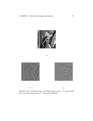
![CHAPTER 2. Discrete-Time Signals and Systems 71
47. MATLAB script:
function y = lccde(b,a,x)
% P0247: LCCDE stream implementation
% Eq.(2.94) y[n] = -sum_{k=1}^N{a_k*y[n-k]}+sum_{k=0}^M{b_k*x[n-k]}
%% Testing:
% b = [0.18 0.1 0.3 0.1 0.18];
% a = [1 -1.15 1.5 -0.7 0.25];
% [x n] = delta(0,0,59);
%% function:
na = length(a); nb = length(b);
if a(1)~=1
a = a/a(1);
end
nab = max([na,nb]);
nx = length(x);
x = [zeros(1,nab-1),x(:)’];
y = zeros(1,nx+nab-1);
for ii = nab:nx+nab-1
y(ii) = b(1)*x(ii);
for jj = 2:nab
y(ii) = y(ii)-a(jj)*y(ii-jj+1)+b(jj)*x(ii-jj+1);
end
end
y = y(end-nx+1:end);
48. Solution:
y(t) = h(t) ∗ x(t) =
∞
−∞
h(τ)x(t − τ)dτ
=
∞
−∞
[u(τ) − u(τ − 3)] [u(t − τ) − u(t − τ − 2)] dτ
=
3
0
[u(t − τ) − u(t − τ − 2)] dτ
0 ≤ t ≤ 2, y(t) =
t
0
1dτ = t
2 ≤ t ≤ 3, y(t) =
t
t−2
1dτ = 2](https://image.slidesharecdn.com/applied-digital-signal-processing-1st-edition-manolakis-solutions-manual-190422092224/85/Applied-Digital-Signal-Processing-1st-Edition-Manolakis-Solutions-Manual-71-320.jpg)
![CHAPTER 2. Discrete-Time Signals and Systems 72
3 ≤ t ≤ 5, y(t) =
3
t−2
1dτ = 5 − t
otherwise, y(t) = 0.
49. Solution:
h(t) = e−t/2
u(t), x(t) = x2(t) = 2, 0 ≤ t ≤ 3
y(t) = x(t) ∗ h(t) =
∞
−∞
h(τ)x(t − τ)dτ
0 ≤ t ≤ 3
y(t) = 2
t
0
e−τ/2
dτ = 4 − 4e−t/2
t ≥ 3
y(t) = 2
t
t−3
e−τ/2
dτ = 4e−t/2
(e3/2
− 1)
y(t) = 0, otherwise
0 1 2 3 4 5 6 7 8 9 10
0
0.5
1
1.5
2
2.5
3
3.5
MSE = 0.008718
t (∆ T = 0.1)
yhat[n]
y[n]
FIGURE 2.65: Plot of sequences ˆy(nT) and y(nT) for T = 0.1.
MATLAB script:](https://image.slidesharecdn.com/applied-digital-signal-processing-1st-edition-manolakis-solutions-manual-190422092224/85/Applied-Digital-Signal-Processing-1st-Edition-Manolakis-Solutions-Manual-72-320.jpg)
![CHAPTER 2. Discrete-Time Signals and Systems 73
0 1 2 3 4 5 6 7 8 9 10
0
0.5
1
1.5
2
2.5
3
3.5
MSE = 8.5688e−05
t (∆ T = 0.01)
yhat[n]
y[n]
FIGURE 2.66: Plot of sequences ˆy(nT) and y(nT) for T = 0.01.
% P0249: Compute and plot continuous-time convolution
% using discrete approximation
close all; clc
% dT = 0.1;
dT = 0.01;
n = 0:10/dT;
t = n*dT;
h = exp(-t/2); % h in P0220
x = zeros(1,length(n));
ind = (t >= 0 & t <=3);
x(ind) = 2; % x2 in P0220
% Theoretical continuous y(t):
y = zeros(1,length(n));
ind = (t >= 0 & t <= 3);
y(ind) = 4-4*exp(-t(ind)/2);
ind = (t >=3);
y(ind) = 4*(exp(1.5)-1)*exp(-t(ind)/2);
% Approximated y(t):
yhat = conv(h,x);](https://image.slidesharecdn.com/applied-digital-signal-processing-1st-edition-manolakis-solutions-manual-190422092224/85/Applied-Digital-Signal-Processing-1st-Edition-Manolakis-Solutions-Manual-73-320.jpg)
![CHAPTER 2. Discrete-Time Signals and Systems 74
yhat = dT*yhat;
yhat = yhat(1:length(n));
% Compute mean square error:
mse = mean((y-yhat).^2);
% Plot:
hf1 = figconfg(’P0249’);
plot(t,yhat,’.’,t,y,’-.’)
TB = [’MSE = ’,num2str(mse)];
title(TB,’fontsize’,TFS)
LB = [’t (Delta T = ’,num2str(dT),’)’];
xlabel(LB,’fontsize’,LFS);
legend(’yhat[n]’,’y[n]’,’location’,’best’)](https://image.slidesharecdn.com/applied-digital-signal-processing-1st-edition-manolakis-solutions-manual-190422092224/85/Applied-Digital-Signal-Processing-1st-Edition-Manolakis-Solutions-Manual-74-320.jpg)
![CHAPTER 2. Discrete-Time Signals and Systems 75
Review Problems
50. MATLAB script:
% P0250: Generate digital reverberation using audio file ’handel’
% and compare it with the one generated in P0219
close all; clc
load(’handel.mat’)
[d nd] = delta(0,0,1e3);
n = 1:length(y);
a = 0.7; % specify attenuation factor
tau = 50e-3; % Part (a)
% tau = 100e-3; % Part (b)
% tau = 500e-3; % Part (c)
D = floor(tau*Fs); % compute delay
yir = filter([zeros(1,length(D)) 1],[1 zeros(1,length(D)-1),-a],d);
% Plot:
hf = figconfg(’P0250’);
plot(nd,yir)
% axis([n(1)-1 n(end)+1 min(y3(1:length(n)))-1 max(y3(1:length(n)))+1])
xlabel(’n’,’fontsize’,LFS);
title(’Impulse Response’,’fontsize’,LFS)
yd = filter([zeros(1,length(D)) 1],[1 zeros(1,length(D)-1),-a],y);
yd_ref = filter(1,[1 zeros(1,length(D)-1),-a],y);
% sound(y,Fs)
% pause(1)
sound(yd,Fs)
pause(1)
sound(yd_ref,Fs)](https://image.slidesharecdn.com/applied-digital-signal-processing-1st-edition-manolakis-solutions-manual-190422092224/85/Applied-Digital-Signal-Processing-1st-Edition-Manolakis-Solutions-Manual-75-320.jpg)
![CHAPTER 2. Discrete-Time Signals and Systems 76
0 100 200 300 400 500 600 700 800 900 1000
0
0.1
0.2
0.3
0.4
0.5
0.6
0.7
0.8
0.9
1
n
Impulse Response
FIGURE 2.67: Impulse response for a = 0.7.
51. (a) Solution:
h[n] ∗ g[n] =
∞
k=0
akδ[n − kD] ∗
∞
l=0
blδ[n − lD]
=
∞
k=0
∞
l=0
akblδ[n − kD] ∗ δ[n − lD]
=
∞
k=0
∞
l=0
akblδ[n − kD − lD]
=
∞
k=0
ckδ[n − kD] = δ[n]
Hence, we can conclude
c0 = a0b0 = 1
ck = k
m=0 ak−mbm = 0, k > 0](https://image.slidesharecdn.com/applied-digital-signal-processing-1st-edition-manolakis-solutions-manual-190422092224/85/Applied-Digital-Signal-Processing-1st-Edition-Manolakis-Solutions-Manual-76-320.jpg)
![CHAPTER 2. Discrete-Time Signals and Systems 77
(b) Solution:
c0 = a0b0 = 1
c1 = a0b1 + a1b0 = 0
c2 = a0b2 + a1b1 + a2b0 = 0
=⇒
b0 = a−1
0
b1 = −a1a−2
0
b2 = −a2a−2
0 + a2
1a−3
0
(c) Solution:
Combined the conditions and the results of previous parts, we have
bk + 0.5bk−1 + 0.25bk−2 = 0, b0 = 1, b1 = −0.5, b2 = 0
k 0 1 2 3 4 5 6 7 · · ·
bk 1 −0.5 0 0.53 −0.54 0 0.56 −0.57 · · ·
We can conclude that
bk =
0.5k, k = 3l
−0.5k, k = 3l + 1
0, k = 3l + 2
l = 0, 1, 2, . . .
52. (a) Solution:
u[n] =
∞
k=0
δ[n − k] =
n
k=−∞
δ[k]
s[n] = h[n] ∗ u[n] = h[n] ∗
∞
k=0
δ[n − k] =
∞
k=0
h[n] ∗ δ[n − k]
=
∞
k=0
h[n − k]
if ∞
k=0 h[n − k] = 0, for all n < 0
∞
k=0 h[−1 − k] = ∞
k=0 h[−2 − k] + h[−1] = 0
∞
k=0 h[−2 − k] = 0
=⇒ h[−1] = 0
Follow the above procedure, we can prove by mathematical induction
that h[n] = 0, for all n < 0. Hence, we conclude a system is causal if
the step response s[n] is zero for n < 0.
(b) Solution:
y[n] = x[n] ∗ h[n] =
∞
m=−∞
h[n − m]x[m]](https://image.slidesharecdn.com/applied-digital-signal-processing-1st-edition-manolakis-solutions-manual-190422092224/85/Applied-Digital-Signal-Processing-1st-Edition-Manolakis-Solutions-Manual-77-320.jpg)
![CHAPTER 2. Discrete-Time Signals and Systems 78
Suppose a period of h[n] is N, that is h[n + N] = h[n].
y[n + N] =
∞
m=−∞
h[N + n − m]x[m] =
∞
m=−∞
h[n − m]x[m] = y[n]
Hence, we proved the output is periodic.
(c) Solution: Wrong. A counter example is the output of the stable system
is always zero.
(d) Solution: Wrong: The inverse of the identity system is itself and it is
causal.
(e) Solution: Wrong. A counter example, h[n] = (0.5)nu[n], is both of
infinite-duration and stable.
(f) Solution: Wrong. A counter example is h[n] = u[n] which is unstable.
53. (a) Solution:
h[n] = δ[n + 1] − 2δ[n] + δ[n − 1]
(b) Comments: The resulting image highlights vertical edges.
(c) Comments: The resulting image highlights horizontal edges.
MATLAB script:
% P0253: Filtering 2D image lena.jpg using 1D second
% derivative filter: y[n] = x[n+1]-2x[n]+x[n-1]
close all; clc
x = imread(’lena.jpg’);
[nx ny] = size(x);
% Part (b): row processing
hfs = figconfg(’P0253a’,’small’);
imshow(x,[])
h = [1 -2 1];
y1 = zeros(nx,ny);
for ii = 1:nx
temp = conv(double(x(ii,:)),h);
y1(ii,:) = temp(2:end-1);
end
hf1 = figconfg(’P0253b’,’small’);
imshow(y1,[])
% Part (c): column processing
y2 = zeros(nx,ny);](https://image.slidesharecdn.com/applied-digital-signal-processing-1st-edition-manolakis-solutions-manual-190422092224/85/Applied-Digital-Signal-Processing-1st-Edition-Manolakis-Solutions-Manual-78-320.jpg)
![CHAPTER 2. Discrete-Time Signals and Systems 79
for ii = 1:ny
temp = conv(double(x(:,ii)),h);
y2(:,ii) = temp(2:end-1);
end
hf2 = figconfg(’P0253c’,’small’);
imshow(y2,[])](https://image.slidesharecdn.com/applied-digital-signal-processing-1st-edition-manolakis-solutions-manual-190422092224/85/Applied-Digital-Signal-Processing-1st-Edition-Manolakis-Solutions-Manual-79-320.jpg)
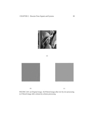
![CHAPTER 2. Discrete-Time Signals and Systems 81
54. (a) Comments: The resulting image is about the fine edge details.
(b) Solution:
h[m, n] =
0 −1 0
−1 5 −1
0 −1 0
(c) Comments: The edge details are enhanced in the resulting image than
the original one.
MATLAB script:
% P0254: Filtering 2D image lena.jpg using 2D Laplacian filter
% Illustrating edge enhancement
close all; clc
% Part (a):
x = imread(’lena.jpg’);
[nx ny] = size(x);
hfs = figconfg(’P0254a’,’small’);
imshow(x,[])
h = [0 1 0;1 -4 1;0 1 0];
y1 = filter2(h,x);
hf1 = figconfg(’P0254b’,’small’);
imshow(y1,[])
% Part (c):
heh = [0 -1 0;-1 5 -1;0 -1 0];
y2 = filter2(heh,x);
hf2 = figconfg(’P0254c’,’small’);
imshow(y2,[])](https://image.slidesharecdn.com/applied-digital-signal-processing-1st-edition-manolakis-solutions-manual-190422092224/85/Applied-Digital-Signal-Processing-1st-Edition-Manolakis-Solutions-Manual-81-320.jpg)
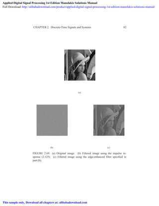


![Digital Signal Processing[ECEG-3171]-Ch1_L02](https://cdn.slidesharecdn.com/ss_thumbnails/dspl2-180427094423-thumbnail.jpg?width=640&height=640&fit=bounds)

![Digital Signal Processing[ECEG-3171]-Ch1_L03](https://cdn.slidesharecdn.com/ss_thumbnails/dspl3-180427094423-thumbnail.jpg?width=640&height=640&fit=bounds)


![RF Circuit Design - [Ch2-1] Resonator and Impedance Matching](https://cdn.slidesharecdn.com/ss_thumbnails/ch2-1-150613064353-lva1-app6892-thumbnail.jpg?width=640&height=640&fit=bounds)


![Circuit Network Analysis - [Chapter4] Laplace Transform](https://cdn.slidesharecdn.com/ss_thumbnails/ch4-150613063858-lva1-app6891-thumbnail.jpg?width=640&height=640&fit=bounds)
![RF Circuit Design - [Ch1-2] Transmission Line Theory](https://cdn.slidesharecdn.com/ss_thumbnails/ch1-2-150613064349-lva1-app6892-thumbnail.jpg?width=640&height=640&fit=bounds)