My talk in the MCQMC Conference 2016, Stanford University. The talk is about Multilevel Hybrid Split Step Implicit Tau-Leap for Stochastic Reaction Networks.

1. Multilevel Hybrid Split Step Implicit Tau-Leap
for Stochastic Reaction Networks (SRNs)
Chiheb Ben Hammouda, Alvaro Moraes and Ra´ul Tempone
MCQMC Conference 2016, Stanford University
August 15, 2016
1/24

2. Outline
1 Introduction
2 Multilevel Hybrid Split Step Implicit Tau-Leap (SSI-TL)
Estimator
3 Numerical Results
2/24

3. SRNs applications: epidemic processes [Anderson and Kurtz, 2015]
and virus kinetics [Hensel et al., 2009],. . .
Biological Models
In-vivo population control: the
expected number of proteins.
Figure 1.1: DNA transcription and
mRNA translation [Briat et al., 2015]
Chemical reactions
the expected number of molecules.
Figure 1.2: Chemical reaction
network [Briat et al., 2015]
3/24

4. Statement of the Forward Problem
A stochastic reaction network (SRN) is a continuous-time Markov Chain X
defined on a probability space (Ω, F, P)
X = (X1, . . . , Xd) : [0, T] × Ω → Zd
+
described by J reactions channels, Rj := (νj, aj), where
νj ∈ Zd
+: stoichiometric vector (state change vector)
aj : Rd
+ → R+: Propensity (jump intensity) functions such that
P X(t + ∆t) = x + νj X(t) = x = aj(x)∆t + o (∆t) , j = 1, . . . , J. (1)
Goal: Given i) an initial state X0 = x0, ii) a smooth scalar observable of X,
g : Rd → R, iii) a user-selected tolerance, TOL, and iv) a confidence level 1 − α
close to 1, provide accurate estimator ˆQ of E [g(X(T))] such that
P E [g(X(T))] − ˆQ < TOL > 1 − α, (2)
with near-optimal expected computational work and for a class of systems
characterized by having simultaneously fast and slow time scales (Stiff systems).
4/24

5. Statement of the Forward Problem
A stochastic reaction network (SRN) is a continuous-time Markov Chain X
defined on a probability space (Ω, F, P)
X = (X1, . . . , Xd) : [0, T] × Ω → Zd
+
described by J reactions channels, Rj := (νj, aj), where
νj ∈ Zd
+: stoichiometric vector (state change vector)
aj : Rd
+ → R+: Propensity (jump intensity) functions such that
P X(t + ∆t) = x + νj X(t) = x = aj(x)∆t + o (∆t) , j = 1, . . . , J. (1)
Goal: Given i) an initial state X0 = x0, ii) a smooth scalar observable of X,
g : Rd → R, iii) a user-selected tolerance, TOL, and iv) a confidence level 1 − α
close to 1, provide accurate estimator ˆQ of E [g(X(T))] such that
P E [g(X(T))] − ˆQ < TOL > 1 − α, (2)
with near-optimal expected computational work and for a class of systems
characterized by having simultaneously fast and slow time scales (Stiff systems).
4/24

6. Simulation of SRNs
Pathwise-Exact methods:
Stochastic simulation algorithm (SSA) [Gillespie, 1976].
Modified next reaction algorithm (MNRA) [Anderson, 2007].
Pathwise-approximate methods:
Explicit tau-leap [Gillespie, 2001, J. Aparicio, 2001].
Drift-implicit tau-leap (explicit-TL) [Rathinam et al., 2003b].
Split step implicit tau-leap (SSI-TL)[Ben Hammouda et al., 2016].
5/24

7. Motivation and Contribution
MLMC estimator using explicit TL [Anderson and Higham, 2012].
In systems characterized by having simultaneously fast and slow
time scales, exact methods and the explicit-TL method can be
very slow and numerically unstable.
We propose in [Ben Hammouda et al., 2016] an efficient MLMC
method that uses SSI-TL approximation at levels where the
explicit-TL method is not applicable due to numerical stability
issues.
6/24

8. The Explicit-TL Method
[Gillespie, 2001, J. Aparicio, 2001]
From Kurtz’s random time-change representation
X(t) = x0 +
J
j=1
Yj
t
t0
λj(X(s))ds νj,
where Yj are independent unit-rate Poisson processes, we obtain the explicit-TL
method (kind of forward Euler approximation): Given Zexp(t) = z ∈ Zd
+,
Zexp
(t + τ) = z +
J
j=1
Pj


aj(z)τ
λj


 νj,
Pj(λj) are independent Poisson random variables with rate λj.
Caveat: The explicit-TL is not adequate when dealing with stiff problems (
Numerical stability ⇒ τexp
threshold 1.)

9. Split Step Implicit Tau-Leap (SSI-TL) Method I
The explicit-TL scheme, where z = Zexp(t), can be rewritten as follows:
Zexp
(t + τ) = z +
J
j=1
Pj (aj(z)τ) νj
= z +
J
j=1
(Pj (aj(z)τ) − aj(z)τ + aj(z)τ) νj
= z +
J
j=1
aj(z)τνj
drift
+
J
j=1
(Pj (aj(z)τ) − aj(z)τ) νj
zero-mean noise
. (3)
8/24

10. Split Step Implicit Tau-Leap (SSI-TL) Method II
The idea of SSI-TL method is to take only the drift part as implicit
while the noise part is left explicit. Let us define z = Zimp(t) and
define Zimp(t + τ) through the following two steps:
y = z +
J
j=1
aj (y) τνj (Drift-Implicit step) (4)
Zimp
(t + τ) = y +
J
j=1
(Pj(aj(y)τ) − aj(y)τ) νj
= z +
J
j=1
Pj(aj(y)τ)νj (Tau-leap step)
9/24

11. Multilevel Monte Carlo by Giles [Giles, 2008]
Goal: Reduce the variance of the standard Monte Carlo estimator.
A hierarchy of nested meshes of the time interval [0, T], indexed by
= 0, 1, . . . , L.
h = M− h0: The size of the subsequent time steps for levels ≥ 1 , where
M>1 is a given integer constant and h0 the step size used at level = 0.
Z : The approximate process generated using a step size of h .
Consider now the following telescoping decomposition of E [g(ZL(T))]:
E [g(ZL(T))] = E [g(Z0(T))] +
L
=1
E [g(Z (T)) − g(Z −1(T))] . (5)
By defining



ˆQ0 := 1
N0
N0
n0=1
g(Z0,[n0](T))
ˆQ := 1
N
N
n =1
g(Z ,[n ](T)) − g(Z −1,[n ](T)) ,
(6)
we arrive at the unbiased MLMC estimator, ˆQ, of E [g(ZL(T))]:
ˆQ :=
L
=0
ˆQ . (7)
10/24

12. Multilevel Hybrid SSI-TL I
Our multilevel hybrid SSI-TL estimator is defined as:
ˆQ := ˆQLimp
c
+
Lint−1
=Limp
c +1
ˆQ + ˆQLint +
L
=Lint+1
ˆQ , (8)
where



ˆQLimp
c
:= 1
N
i,L
imp
c
N
i,L
imp
c
n=1
g(Zimp
Limp
c ,[n]
(T))
ˆQ := 1
Nii,
Nii,
n =1
g(Zimp
,[n ](T)) − g(Zimp
−1,[n ](T)) , Limp
c + 1 ≤ ≤ Lint − 1
ˆQLint := 1
Nie,Lint
Nie,Lint
n=1
g(Zexp
Lint,[n]
(T)) − g(Zimp
Lint−1,[n]
(T))
ˆQ := 1
Nee,
Nee,
n =1
g(Zexp
,[n ](T)) − g(Zexp
−1,[n ](T)) , Lint + 1 ≤ ≤ L.
(9)
11/24

13. Multilevel Hybrid SSI-TL II
1 Limp
c , the coarsest discretization level.
2 Lint, the interface level.
3 L, the finest discretization level.
4 N := {Ni,Limp
c
, {Nii, }Lint−1
=Limp
c +1
, Nie,Lint , {Nee, }L
=Lint+1
}, the number of
samples per level.
The expected computational cost of the MLMC estimator given that the
interface level is Lint, given by
WLint := Ci,Limp
c
Ni,Limp
c
h−1
Limp
c
+
Lint−1
=Limp
c +1
Cii, Nii, h−1
+ Cie,Lint Nie,Lint h−1
Lint +
L
=Lint+1
Cee, Nee, h−1
, (10)
where Ci, Cii, Cie and Cee are, respectively, the expected computational costs
of simulating a single SSI-TL step, a coupled SSI-TL step, a coupled
SSI/explicit TL step and a coupled explicit-TL step.
12/24

14. Explicit-TL/Explicit-TL Coupling (Idea)
[Kurtz, 1982, Anderson and Higham, 2012]
To couple two Poisson random variables, P1(λ1), P2(λ2), with rates λ1 and
λ2, respectively, we define λ := min{λ1, λ2} and we consider the
decomposition
P1(λ1) := Q(λ ) + Q1(λ1 − λ )
P2(λ2) := Q(λ ) + Q2(λ2 − λ )
where Q(λ ), Q1(λ1 − λ ) and Q2(λ2 − λ ) are three independent Poisson
random variables.
We have small variance between the coupled processes
Var [P1(λ1) − P2(λ2)] = Var Q1(λ1 − λ ) − Q2(λ2 − λ )
=| λ1 − λ2 | .
Observe: If P1(λ1) and P2(λ2) are independent, then, we have a larger variance
Var [P1(λ1) − P2(λ2)] = λ1 + λ2.

15. Estimation procedure I
Coarsest discretization level, Limp
c , is determined by the numerical
stability constraint of our MLMC estimator, two conditions must be
satisfied:
The stability of a single path: determined by a linearized stability
analysis of the backward Euler method applied to the
deterministic ODE model corresponding to our system.
The stability of the variance of the coupled paths of our MLMC
estimator: expressed by
Var g(ZLimp
c +1
)−g(ZLimp
c
) Var g(ZLimp
c
) .
14/24

16. Estimation procedure II
Total number of levels, L, and the set of the number of samples
per level, N, are selected to satisfy the accuracy constraint given by
(2), with near-optimal expected computational work. As a result, the
MLMC algorithm should bound the bias and the statistical error as
follows:
E g(X(T)) − ˆQ ≤ (1 − θ) TOL, (11)
Var ˆQ ≤
θ TOL
Cα
2
(12)
for some given confidence parameter, Cα, such that Φ(Cα) = 1 − α/2 ;
here, Φ is the cumulative distribution function of a standard normal
random variable.
15/24

17. Estimation procedure III
In our problem, the finest discretization level, L, is determined by
satisfying relation (11) for θ = 1
2, implying
|Bias(L) := E [g(X(T)) − g(ZL(T))]| <
TOL
2
. (13)
In our numerical experiments, we use the following approximation (see
[Giles, 2008])
Bias(L) ≈ E [g(ZL(T)) − g(ZL−1(T))] . (14)
16/24

18. Estimation procedure IV
The interface level, Lint and optimal number of samples per level, N
are determined by the following two steps:
1 The first step is to solve (15), for a fixed value of the interface level, Lint



min
N
WLint (N)
s.t. Cα
L
=Limp
c
N−1
V ≤ TOL
2 ,
(15)
where V = Var [g(Z (T)) − g(Z −1(T)] is estimated by the extrapolation
of the sample variances obtained from the coarsest levels (due to the
presence of large kurtosis.
2 Let us denote N∗(Lint) as the solution of (15). Then, the optimal value of
the switching parameter, Lint, should be chosen to minimize the expected
computational work; that is, the value Lint∗
that solves



min
Lint
WLint (N∗(Lint))
s.t. Lexp
c ≤ Lint ≤ L.
For this method, the lowest computational cost is achieved for
Lint∗
= Lexp
c , i.e., the same level in which the explicit-TL is stable.
17/24

19. Multilevel Hybrid SSI-TL: Results I
This example was studied in [Rathinam et al., 2003a] and is given by the
following reaction set
S1
c1
→ S3,
S3
c2
→ S1
S1 + S2
c3
→ S1 + S4. (16)
The corresponding propensity functions are
a1(X) = c1X1, a2(X) = c2(K − X1), a3(X) = c3X1X2.
where K = X1 + X3.
c = (c1, c2, c3) = (105, 105, 5 × 10−3), X(0) = (104, 102) and K = 2.104.
We are interested in approximating E [X2(T)], where T = 0.01 seconds.
This setting implies that the stability limit of the explicit-TL is
τlim
exp ≈ 10−5.
17/24

20. Multilevel Hybrid SSI-TL: Results II
Method / TOL 0.02 0.01 0.005
Multilevel explicit-TL 890 (9) 5300 (45) 2.2e+04 (96)
Multilevel SSI-TL 240 (0.8) 110 (3) 5.3e+02 (7)
Wexp
MLMC/WSSI
MLMC 37.04 47.33 41.27
Table 1: Comparison of the expected total work for the different methods (in
seconds) using 100 multilevel runs. (·) refers to the standard deviation. The
last row shows that the multilevel SSI-TL estimator outperforms by about 40
times the multilevel explicit-TL estimator in terms of computational work.
18/24

21. Multilevel Hybrid SSI-TL: Results III
10
−3
10
−2
10
−1
10
0
10
2
10
4
10
6
10
8
Comparison of the expected total work for the different methods for different values of tolerance TOL
TOL
Expectedtotalwork(W)(seconds)
Multilevel SSI−TL (L
c
imp
=0)
Linear reference with slope −2.25
Multilevel explicit TL (Lc
exp
=11)
Linear reference with slope −2.37
MC SSI−TL
Linear reference with slope −2.77
y=TOL−2
(log(TOL))2
y=TOL
−3
Figure 3.1: Comparison of the expected total work for the different methods
with different values of tolerance (TOL) using 100 multilevel runs. The
computational work, W, of both multilevel SSI-TL and multilevel explit-TL
methods is of O TOL−2
(log(TOL))2
compared to O TOL−3
for the MC
SSI-TL.
19/24

22. Multilevel Hybrid SSI-TL: Results IV
10
−3
10
−2
10
−1
10
−4
10
−3
10
−2
10
−1
TOL
Totalerror
TOL vs. Global error
1 %
1 %
2 %
5 %
Figure 3.2: TOL versus the actual computational error. The numbers above
the straight line show the percentage of runs that had errors larger than the
required tolerance.
20/24

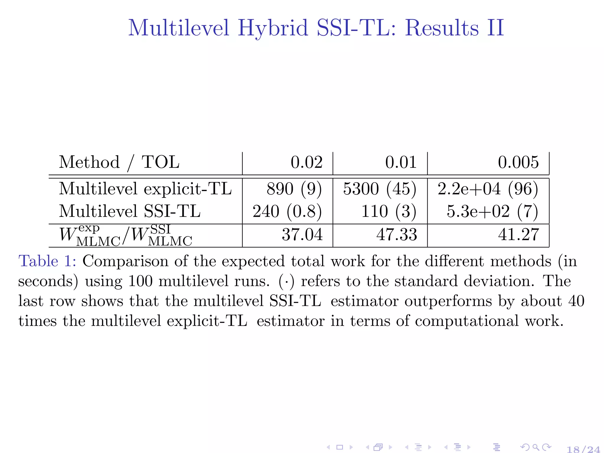
23. Summary
Our proposed estimator is useful in systems with the presence of
slow and fast timescales (stiff systems): obtained substantial gains
with respect to both the multilevel explit-TL
[Anderson and Higham, 2012].
For large values of TOL, the multilevel SSI-TL method has the
same order of computational work as does the multilevel explit-TL
method (O TOL−2 log(TOL)2 ) [Anderson et al., 2014], but with
a smaller constant.
21/24

24. Future work
Implementing Hybridization techniques involving methods that
deal with non-negativity of species [Moraes et al., 2015b] and
adaptive methods introduced in [Karlsson and Tempone, 2011,
Moraes et al., 2015a, Lester et al., 2015], which allows us to
construct adaptive hybrid multilevel estimators by switching
between SSI-TL, explicit-TL and exact SSA.
Extending the τ-ROCK method [Abdulle et al., 2010] to the
multilevel setting and compare it with the multilevel hybrid
SSI-TL method. The main challenge of this task is to couple two
consecutive paths based on the τ-ROCK method.
Addressing spatial inhomogeneities described, for instance, by
graphs and/or continuum volumes through the use of Multi-Index
Monte Carlo technology [Haji-Ali et al., 2015].
22/24

25. References I
Abdulle, A., Hu, Y., and Li, T. (2010).
Chebyshev methods with discrete noise: the tau-rock methods.
J. Comput. Math, 28(2):195–217.
Anderson, D. and Higham, D. (2012).
Multilevel Monte Carlo for continuous Markov chains, with
applications in biochemical kinetics.
SIAM Multiscal Model. Simul., 10(1).
Anderson, D. F. (2007).
A modified next reaction method for simulating chemical systems
with time dependent propensities and delays.
The Journal of Chemical Physics, 127(21):214107.
Anderson, D. F., Higham, D. J., and Sun, Y. (2014).
Complexity of multilevel Monte Carlo tau-leaping.
52(6):3106–3127.
23/24

26. References II
Anderson, D. F. and Kurtz, T. G. (2015).
Stochastic analysis of biochemical systems.
Springer.
Ben Hammouda, C., Moraes, A., and Tempone, R. (2016).
Multilevel hybrid split-step implicit tau-leap.
Numerical Algorithms, pages 1–34.
Brauer, F. and Castillo-Chavez, C. (2011).
Mathematical Models in Population Biology and Epidemiology
(Texts in Applied Mathematics).
Springer, 2nd edition.
Briat, C., Gupta, A., and Khammash, M. (2015).
A Control Theory for Stochastic Biomolecular Regulation.
Paris. SIAM.
24/24

27. References III
Giles, M. (2008).
Multi-level Monte Carlo path simulation.
Operations Research, 53(3):607–617.
Gillespie, D. T. (1976).
A general method for numerically simulating the stochastic time
evolution of coupled chemical reactions.
Journal of Computational Physics, 22:403–434.
Gillespie, D. T. (2001).
Approximate accelerated stochastic simulation of chemically
reacting systems.
Journal of Chemical Physics, 115:1716–1733.
Haji-Ali, A.-L., Nobile, F., and Tempone, R. (2015).
Multi-index monte carlo: when sparsity meets sampling.
Numerische Mathematik, pages 1–40.
25/24

28. References IV
Hensel, S., Rawlings, J., and Yin, J. (2009).
Stochastic kinetic modeling of vesicular stomatitis virus
intracellular growth.
Bulletin of Mathematical Biology, 71(7):1671–1692.
J. Aparicio, H. S. (2001).
Population dynamics: Poisson approximation and its relation to
the langevin process.
Physical Review Letters, page 4183.
Karlsson, J. and Tempone, R. (2011).
Towards automatic global error control: Computable weak error
expansion for the tau-leap method.
Monte Carlo Methods and Applications, 17(3):233–278.
26/24

29. References V
Kurtz, T. (1982).
Representation and approximation of counting processes.
In Advances in Filtering and Optimal Stochastic Control,
volume 42 of Lecture Notes in Control and Information Sciences,
pages 177–191. Springer Berlin Heidelberg.
Lester, C., Yates, C. A., Giles, M. B., and Baker, R. E. (2015).
An adaptive multi-level simulation algorithm for stochastic
biological systems.
The Journal of chemical physics, 142(2):024113.
Moraes, A., Tempone, R., and Vilanova, P. (2015a).
Multilevel adaptive reaction-splitting simulation method for
stochastic reaction networks.
preprint arXiv:1406.1989.
27/24

30. References VI
Moraes, A., Tempone, R., and Vilanova, P. (2015b).
Multilevel hybrid chernoff tau-leap.
BIT Numerical Mathematics, pages 1–51.
Rathinam, M., Petzold, L., Cao, Y., and Gillespie, D. T. (2003a).
Stiffness in stochastic chemically reacting systems: the implicit
tau-leaping method.
Journal of Chemical Physics, 119(24):12784–12794.
Rathinam, M., Petzold, L. R., Cao, Y., and Gillespie, D. T.
(2003b).
Stiffness in stochastic chemically reacting systems: The implicit
tau-leaping method.
The Journal of Chemical Physics, 119(24):12784–12794.
28/24

31. References VII
Srivastava, R., You, L., Summers, J., and Yin, J. (2002).
Stochastic vs. deterministic modeling of intracellular viral kinetics.
Journal of Theoretical Biology, 218(3):309–321.
29/24

32. Thank you for your attention
30/24