The document contains details about experiments performed in a Digital Signal Processing practical course. It includes the aims, apparatus required, theory, source code and results for experiments involving MATLAB programs to generate basic signals like impulse, step, ramp and exponential signals; sine and cosine signals; quantization; sampling theorem; linear convolution; autocorrelation; and cross-correlation. Programs were written in MATLAB to perform the various digital signal processing tasks and the output was verified.

1. JAWAHAR LAL NEHRU GOVERNMENT ENGINEERING
COLLEGE
SUNDERNAGAR (175018)
PRACTICAL FILE
OF
DIGITAL SIGNAL PROCESSING
EC- 413(P)
SUBMITTED TO: SUBMITTED BY:
ER. MUNISH BHARDWAJ RAKESH KUMAR THAKUR
BT-30663
7TH
SEMESTER

3. INDEX
S.No. Experiment Remarks
1. Introduction to Matlab 4-7
2. Representation of basic
signal
8-11
3. Representation of
sinusoidal signals
12-15
4. To study Quantization
technique
16-19
5. To study sampling theorem 20-23
6. To develop program for
linear convulation
24-27
7. To develop program for
autocorrelation
28-31
8. To develop program for
cross-correlation
32-35
9. To study ASK,FSK and
PSK
36-41
10. To study window
Technique
42-45
11. To generate triangular and
square wave
46-49

4. EXPERIMENT- 1
AIM:
Introduction to MATLAB

5. EXPERIMENT- 1
AIM:
Introduction to MATLAB
THEORY:
Introduction to MATLAB
Matlab is an interpreted language for numerical computation. It allows one to
perform numerical calculations, and visualize the results without the need for
complicated and time consuming programming. Matlab allows its users to
accurately solve problems, produce graphics easily and produce code efficiently.
MATLAB programs are stored as plain text in files having names that end
with the extension “m”. These files are called m-files. MATLAB functions have
two parameter lists, one for input and one for output. One nifty difference
between MATLAB and traditional high level languages is that MATLAB
functions can be used interactively. In addition to providing the obvious support
for interactive calculation, it also is a very convenient way to debug functions that
are part of a bigger project.
Windows:
 Command Window:
The window where we type commands and non-graphic output is displayed.
A ‘>>’ prompt shows the system is ready for input. The lower left hand corner
of the main window also displays ‘ready’ or ‘Busy’ when the system is waiting
or calculating. Previous commands can be accessed using the up arrow to save
typing and reduce errors. Typing a few characters restricts this function to
commands beginning with those characters.
 Figure Window:
MATLAB directs graphics output to a window that is separate from the
command window. In MATLAB, this window is referred to as a figure. Graphics
functions automatically create new figure windows if none currently exist. If a
figure window already exists, MATLAB uses that window. If multiple figure
windows exist, one is designated as the current figure and is used by MATLAB.
 Editor Window:
The window where we edit m-files the files that hold scripts and functions
that we’ve defined or are editing. Multiple files are generally opened as tabs in
the same editor window, but they can also be tiled for side by side comparison.
Orange warnings and red errors appear as underlining and as bars in the margin.
Covering over them provides more information/clicking on the bar takes us to the

7. Relevant bit of text. Also MATLAB runs the last saved version of a file, so we
have to save before any changes take effect.
Commands:
clc:
Clears command window
clear all:
Deletes all variables from current workspace
close all:
Closes all open figure windows
for (loop):
Iterates over procedure incrementing i by 1
Subplot:
Divide the plot window up into pieces
Stem:
Plot discrete sequence data
Plot:
 plot(x,y):
Plot the elements of vector y (on the vertical axis of a figure) versus the
elements of the vector x (on the horizontal axis of the figure).
 plot(w,abs(y)):
Plot the magnitude of vector y (on the vertical axis of a figure) versus
the elements of the vector w (on the horizontal axis of the figure).
 plot(w,angle(y)):
Plot the phase of vector y in radian (on the vertical axis of a figure)
versus the elements of the vector w (on the horizontal axis of the figure).
Label:
 X label:
Add a label to the horizontal axis of the current plot.
 Y label:
Add a label to the vertical axis of the current plot.
Title:
Add a title to the current plot

8. EXPERIMENT- 2
AIM:
Write a program in MATLAB to generate the following waveforms:
Unit impulse signal, Unit step signal, Ramp signal, Exponential signal;
APPARATUS REQUIRED:
Computer, MATLAB software;

9. EXPERIMENT- 2
AIM:
Write a program in MATLAB to generate the following waveforms:
Unit impulse signal, Unit step signal, Ramp signal, Exponential signal;
APPARATUS REQUIRED:
Computer, MATLAB software;
THEORY:
Real signals can be quite complicated. The study of signals therefore starts with
the analysis of basic and fundamental signals. For linear systems, a complicated
signal and its behaviour can be studied by superposition of basic signals.
Common basic signals are:
Discrete – Time signals:
 Unit impulse sequence.
 Unit step sequence.
 Unit ramp sequence.
 Exponential sequence. x(n) = A an
, where A and a are constant
SOURCE CODE:
%WAVE FORM GENERATION
%UNIT IMPULSE
clc; clear all; close all;
n1 = -3:1:3;
x1 = [0,0,0,1,0,0,0];
subplot(2,2,1);
stem(n1,x1);
xlabel('time');
ylabel('Amplitude');
x n n
n
( ) ( )
,
 




1 0
0
for
, otherwise
x n u n
n
( ) ( )
,
 



1 0
0
for
, otherwise
x n r n
n n
( ) ( )
,
 



for
, otherwise
0
0

10. RESULT:
The program to generate various waveforms is written, executed and the output
is verified

11. title('Unit impulse signal');
%UNIT STEP SIGNAL
n2=-5:1:25;
x2=[zeros(1,5),ones(1,26)];
subplot(2,2,2);
stem(n2,x2);
xlabel('time');
ylabel('Amplitude');
title('Unit step signal');
%EXPONENTIAL SIGNAL
a=5;
n3=-10:1:20;
x3=power(a,n3);
subplot(2,2,3);
stem(n3,x3);
xlabel('time');
ylabel('Amplitude');
title('Exponential signal');
%UNIT RAMP SIGNAL
n4=-10:1:20;
x4=n4;
subplot(2,2,4);
stem(n4,x4);
xlabel('time');
ylabel('Amplitude');
title('Unit ramp signal');
RESULT:
The program to generate various waveforms is written, executed and the output
is verified.

12. EXPERIMENT- 3
AIM:
Write a program in MATLAB to generate the following waveforms:
Sine and Cosine signal;
APPARATUS REQUIRED:
Computer, MATLAB software;

13. EXPERIMENT- 3
AIM:
Write a program in MATLAB to generate the following waveforms:
Sine and Cosine signal;
APPARATUS REQUIRED:
Computer, MATLAB software;
THEORY:
Real signals can be quite complicated. The study of signals therefore starts with
the analysis of basic and fundamental signals. For linear systems, a complicated
signal and its behaviour can be studied by superposition of basic signals.
Common basic signals are:
Sinusoidal signal.
SOURCE CODE:
%WAVE FORM GENERATION
%SINE SIGNAL
A=input('Enter the amplitude:');
f=input('Enter the frequency:');
n1=-pi:0.03:pi;
x1=A*sin(2*f*n1);
subplot(2,1,1);
stem(n1,x1);
xlabel('time');
ylabel('Amplitude');
title('Sine signal');
%COSINE SIGNAL
x t A( ) sin( ) t



14. RESULT:
The program to generate various waveforms is written, executed and the output
is verified.

15. A=input('Enter the amplitude:');
f=input('Enter the frequency:');
n2=-pi:0.03:pi;
x2=A*cos(2*f*n2);
subplot(2,1,2);
stem(n2,x2);
xlabel('time');
ylabel('Amplitude');
title('Cosine signal');
RESULT:
The program to generate various waveforms is written, executed and the output
is verified.

16. EXPERIMENT- 4
AIM:
To develop program for quantization
APPARATUS REQUIRED:
PC, MATLAB software

17. EXPERIMENT- 4
AIM:
To develop program for quantization
APPARATUS REQUIRED:
PC, MATLAB software
THEORY:
Quantization:
A continuous time signal, such as voice, has a continuous range of amplitudes
and therefore its samples have a continuous amplitude range i.e. they are only
discrete in time not in amplitude. In other words, within the finite amplitude range
of the signal, we find an infinite number of amplitude levels. It is not necessary
in fact to transmit the exact amplitude of the samples. Any human sense (the ear
or the eye), as ultimate receiver, can detect only finite intensity differences. This
means that the original continuous time signal may be approximated by a signal
constructed of discrete amplitudes selected on a minimum error basis from an
available set. Clearly, if we assign the discrete amplitude levels with sufficiently
close spacing we may take the approximated signal practically indistinguishable
from the original continuous signal.
Amplitude quantization is defined as the process of transforming
the sample amplitude m(nTs) of a message signal m(t) at time t=nTs into a
discrete amplitude v(nTs) taken from a finite set of possible amplitudes.
SOURCE CODE:
%MATLAB code for ask fsk and psk
clc;
clear all;
close all;
%input signal
t=0:0.1:2*pi;
y=sin(t);
%quantizing input signal
z=round(y);
%ploting signals
plot(y);
hold all;
stem(y,'g');
hold all;
stem(z,'r');
hold all;

18. RESULT:
The quantization is performed by using MATLAB script

19. xlabel('time');
ylabel('Amplitude');
title('Quantization');
RESULT:
The quantization performed by using MATLAB script

20. EXPERIMENT- 5
AIM:
To understand sampling theorem.
APPARATUS REQUIRED:
PC, MATLAB software

21. EXPERIMENT- 5
AIM:
To understand sampling theorem.
APPARATUS REQUIRED:
PC, MATLAB software
THEORY:
SAMPLING PROCESS:
It is a process by which a continuous time signal is converted into discrete
time signal. X[n] is the discrete time signal obtained by taking samples of the
analog signal x(t) every T seconds, where T is the sampling period.
X[n] = x (t) x p (t)
Where p(t) is impulse train; T – period of the train
SAMPLING THEOREM:
It states that the band limited signal x(t) having no frequency components
above Fmax Hz is specified by the samples that are taken at a uniform rate greater
than 2 Fmax Hz (Nyquist rate), or the frequency equal to twice the highest
frequency of x(t).
Fs ≥ 2 Fmax
SOURCE CODE:
clc;
clear all;
close all;
%continuous sinusoidal signal
a=input('Enter the amplitude :');
f=input('Enter the Timeperiod :');
t=-pi:0.3:pi;

22. RESULT:
The sampling theorem performed by using MATLAB script

23. x=a*sin(2*f*t);
subplot(4,1,1);
plot(t,x);
xlabel('time');ylabel('Amplitude');
title('Sinusoidal signal');
%sampling without distortion
fs=input('enter sampling frequency(fs=>2*f) : ');
y=a*sin(2*f*fs*t);
subplot(4,1,2);
plot(t,y);
xlabel('time');
ylabel('Amplitude');
title('Distortion less Sinusoidal signal');
%critical sampling
fs=input('enter sampling frequency fs=2*f : ');
z=a*sin(2*f*fs*t);
subplot(4,1,3);
plot(t,z);
xlabel('time');
ylabel('Amplitude');
title('Sampled at Nyquist rate Sinusoidal signal');
%sampling with distortion
fs=input('enter sampling frequency fs=2*f : ');
u=a*sin(2*f*fs*t);
subplot(4,1,4);
plot(t,u);
xlabel('time');
ylabel('Amplitude');
title('Distorted Sinusoidal signal');
RESULT:
The sampling theorem performed by using MATLAB script

24. EXPERIMENT- 6
AIM:
Write a MATLAB Script to perform discrete convolution (Linear) for the given
two sequences.
APPARATUS REQUIRED:
PC, MATLAB software

25. EXPERIMENT- 6
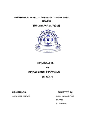
AIM:
Write a MATLAB Script to perform discrete convolution (Linear) for the given
two sequences.
APPARATUS REQUIRED:
PC, MATLAB software
THEORY:
LINEAR CONVOLUTION:
The response y[n] of a LTI system for any arbitrary input x[n] is given by
convolution of impulse response h[n] of the system and the arbitrary input x[n].
y[n] = x[n]*h[n] = 



k
knhkx ][][ or 



k
knxkh ][][
If the input x[n] has N1 samples and impulse response h[n] has N2 samples then
the output sequence y[n] will be a finite duration sequence consisting of (N1 + N2
- 1) samples.
SOURCE CODE:
clc;
clear all;
close all;
%Program to perform Linear Convolution
x1=input('Enter the first sequence to be convoluted:');
subplot(3,1,1);
stem(x1);
xlabel('Time');
ylabel('Amplitude');
title('First sequence');
x2=input('Enter the second sequence to be convoluted:');

26. RESULT:
The linear convolutions are performed by using MATLAB script;

27. subplot(3,1,2);
stem(x2);
xlabel('Time');
ylabel('Amplitude');
title('Second sequence');
f=conv(x1,x2);
disp('The Linear convoluted sequence is');
disp(f);
subplot(3,1,3);
stem(f);
xlabel('Time');
ylabel('Amplitude');
title('Linear Convoluted sequence');
RESULT:
The linear convolutions are performed by using MATLAB script;

28. EXPERIMENT- 7
AIM:
To develop program for autocorrelation
APPARATUS REQUIRED:
PC, MATLAB software

29. EXPERIMENT- 7
AIM:
To develop program for autocorrelation
APPARATUS REQUIRED:
PC, MATLAB software
THEORY:
AUTOCORRELATION:
Autocorrelation is the cross-correlation of a signal with itself.
Informally, it is the similarity between observations as a function of the time
lag between them. It is a mathematical tool for finding repeating patterns,
such as the presence of a periodic signal obscured by noise,
or identifying the missing fundamental frequency in a signal implied by its
harmonic fre3uencies. It is often used in signal processing for analyzing functions
or series of values, such as time domain signals.
SOURCE CODE:
clc;
clear all;
x = input(‘enter the finite length signal sequence’);
N = 0:length(x)-1;
%perform autocorrelation using corr function
y = xcorr(x,x);
%generating time index for the autocorrelation sequence
N2 = -length(x)+1:length(x)-1;
%plot original signal and autocorrelation sequence
subplot(2,1,1);
stem(N,x);
xlabel('N');
ylabel('x(n)');
title('original signal');
subplot(2,1,1);
stem(N2,y);
xlabel('N');
ylabel('y(n)');

30. RESULT:
The autocorrelation is performed by using MATLAB script;

31. title('Autocorrelation signal');
RESULT:
The autocorrelation is performed by using MATLAB script;

32. EXPERIMENT- 8
AIM:
To perform cross-correlation of a given sequence.
APPARATUS REQUIRED:
PC, MATLAB software

33. EXPERIMENT- 8
AIM:
To perform cross-correlation of a given sequence.
APPARATUS REQUIRED:
PC, MATLAB software
THEORY:
CROSS-CORRELATION:
In signal processing, cross-correlation is a measure of similarity of two
waveforms as a function of a time lag applied to one of them. This is also known
as a sliding dot product or sliding inner product. It is commonly used for
searching a long signal for a shorter, known feature. It has applications
in pattern recognition, single particle analysis, electron tomographic
averaging;
The cross-correlation is similar in nature to the convolution of two
functions. In an autocorrelation, which is the cross-correlation of a signal with
itself, there will always be a peak at a lag of zero unless the signal is a trivial zero
signal. In probability theory and statistics, correlation is always used to include a
standardizing factor in such a way that correlations have values between -1 and
+1, and the term cross-correlation is used for referring to the correlation
corr(X,Y), between two random variables X and Y, while the “correlation” of a
random vector X is considered to be the correlation matrix (matrix of
correlations) between the scalar elements of X.
SOURCE CODE:
clc;
clear all;
x1 = input('enter 1st the finite length signal sequence x1(n) : ');
n1 = 0:length(x1)-1;
x2 = input('enter 2nd the finite length signal sequence x2(n) : ');
n2 = 0:length(x2)-1;
%perform cross-correlation using corr function
y12 = xcorr(x1,x2);
y21 = xcorr(x2,x1);
%generating time index for the cross correlation sequence
N1 = -length(x1)+1:length(x1)-1;
N2 = -length(x2)+1:length(x2)-1;

34. RESULT:
The cross-correlation are performed by using MATLAB script;

35. %plot original signal and cross correlation sequence
subplot(4,1,1);
stem(n1,x1);
xlabel('N');
ylabel('x1(n)');
title('original signal x1(n)');
subplot(4,1,2);
stem(n2,x2);
xlabel('N');
ylabel('x2(n)');
title('original signal x2(n)');
subplot(4,1,3);
stem(y12);
xlabel('N1');
ylabel('y12(n)');
title('Cross-correlated sequence');
subplot(4,1,4);
stem(y21);
xlabel('N2');
ylabel('y21(n)');
title('Cross-correlated sequence');
RESULT:
The cross-correlation are performed by using MATLAB script;

36. EXPERIMENT- 9
AIM:
To develop program for ASK, FSK and PSK on Matlab script.
APPARATUS REQUIRED:
PC, MATLAB software

37. EXPERIMENT- 9
AIM:
To develop program for ASK, FSK and PSK on Matlab script.
APPARATUS REQUIRED:
PC, MATLAB software
THEORY:
 Amplitude shift keying
ASK is a modulation process, which imparts to a sinusoid two or more discrete
amplitude levels. These are related to the number of levels adopted by the digital
message. For a binary message sequence there are two levels, one of which is
typically zero. The data rate is a sub-multiple of the carrier frequency. Thus the
modulated waveform consists of bursts of a sinusoid. One of the disadvantages
of ASK, compared with FSK and PSK, is that it has not got a constant envelope.
This makes its processing (e.g., power amplification) more difficult, since
linearity becomes an important factor. However, it does make for ease of
demodulation with an envelope detector.
 Phase-shift keying (FSK)
PSK is a digital modulation scheme that conveys data by changing, or
modulating, the phase of a reference signal (the carrier wave). PSK uses a finite
number of phases, each assigned a unique pattern of binary digits. Usually, each
phase encodes an equal number of bits. Each pattern of bits forms the symbol that
is represented by the particular phase. The demodulator, which is designed
specifically for the symbol-set used by the modulator, determines the phase of the
received signal and maps it back to the symbol it represents, thus recovering the
original data.
In a coherent binary PSK system, the pair of signal S1(t) and S2 (t) used to
represent binary symbols 1 & 0 are defined by
S1 (t) = √2E/ Tb Cos 2πfct
S2 (t) =√2E/Tb (2πfct+π) = - √ 2Eb/Tb Cos 2πfct
where 0 ≤ t< Tb and E = Transmitted signed energy for bit
The carrier frequency fc =n/Tb for some fixed integer n.

39.  Frequency-shift keying (FSK)
Frequency-shift keying (FSK) is a frequency modulation scheme in
which digital information is transmitted through discrete frequency
changes of a carrier wave. The simplest FSK is binary FSK (BFSK). BFSK
uses a pair of discrete frequencies to transmit binary (0s and 1s)
information. With this scheme, the "1" is called the mark frequency and
the "0" is called the space frequency.
In binary FSK system, symbol 1 & 0 are distinguished from each other by
transmitting one of the two sinusoidal waves that differ in frequency by a fixed
amount.
Si (t) = √2E/Tb cos 2πfit 0≤ t ≤Tb
0 elsewhere
Where i=1, 2
E=Transmitted energy/bit
Transmitted freq= ƒi = (nc+i)/Tb, and n = constant (integer),Tb = bit interval
Symbol 1 is represented by S1 (t) Symbol 0 is represented by S0 (t)
SOURCE CODE:
%MATLAB code for ask fsk and psk
clc;
clear all;
f=5;
f2=10;
x=[1 1 0 0 1 0 1 0] ; % input signal
n=length(x);
i=1;
while i<n+1
t = i:0.001:i+1;
if x(i)==1
ask=sin(2*pi*f*t);
fsk=sin(2*pi*f*t);
psk=sin(2*pi*f*t);
else
ask=0;
fsk=sin(2*pi*f2*t);
psk=sin(2*pi*f*t+pi);
end

40. RESULT:
The ASK, FSK, PSK studied and are performed by using MATLAB script;

41. subplot(3,1,1);
plot(t,ask);
hold on;
ylabel ('Amplitude');
xlabel ('Time');
title('Amplitude Shift Key');
subplot(3,1,2);
plot(t,fsk);
hold on;
ylabel ('Amplitude');
xlabel ('Time');
title('Frequency Shift Key')
subplot(3,1,3);
plot(t,psk);
hold on;
ylabel ('Amplitude');
xlabel ('Time');
title('Phase Shift Key')
i=i+1;
end
RESULT:
The ASK, FSK, PSK studied and are performed by using MATLAB script;

42. EXPERIMENT- 10
AIM:
To study different window techniques
APPARATUS REQUIRED:
PC, MATLAB software

43. EXPERIMENT- 10
AIM:
To study different window techniques
APPARATUS REQUIRED:
PC, MATLAB software
THEORY:
Most digital signals are infinite, or sufficiently large that the dataset cannot be
manipulated as a whole. Sufficiently large signals are also difficult to analyze
statistically, because statistical calculations require all points to be available for
analysis. In order to avoid these problems, engineers typically analyze small
subsets of the total data, through a process called windowing
Consider the system H(z), with input X(z) and output Y(z). We model this as:
If we have a window with transfer function W(z), we can mathematically apply
the window to our signal, X(z) as such:
Then, we can pass our windowed signal into our system, H(z) as usual:
w = rectwin(L) returns a rectangular window of length L in the column vector w.
This function is provided for completeness; a rectangular window is equivalent
to no window at all.
w = hamming(L) returns an L-point symmetric Hamming window in the column
vector w. L should be a positive integer. The coefficients of a Hamming window
are computed from the following equation.
w(n)=0.54−0.46cos(2πnN), 0≤n≤N
The window length is L=N+1
w = bartlett(L) returns an L-point Bartlett window in the column vector w, where
L must be a positive integer. The coefficients of a Bartlett window are computed
as follows:

44. RESULT:
The window techniques studied and are generated by using MATLAB
script

45. w(n)=
2n/N
2−2nN
0≤n≤N2
N2≤n≤N
The window length L=N+1
w = blackman(N) returns the N-point symmetric Blackman window in the column
vector w, where N is a positive integer. The following equation defines the
Blackman window of length N:
w(n)=0.42−0.5cos2πnN−1+0.08cos4πnN−1, 0≤n≤M−1
where M is N/2 for N even and (N + 1)/2 for N odd.
SOURCE CODE:
%Program to generate window
%rectangular window
L=10;
w1=rectwin(L);
wvtool(w);
%%
%bartlett window
L=64;
w2=bartlett(L);
wvtool(w2);
%%
%hamming window
L=64;
w3=hamming(L);
wvtool(w3);
%%
%blackman window
L=64;
w4=blackman(L);
wvtool(w4);
RESULT:
The window techniques studied and are generated by using MATLAB
script

46. EXPERIMENT- 11
AIM:
To generate a triangular and square waveform.
APPARATUS REQUIRED:
PC, MATLAB software

47. EXPERIMENT- 11
AIM:
To generate a triangular and square waveform.
APPARATUS REQUIRED:
PC, MATLAB software
THEORY:
SQUARE WAVE:
Square wave is a non-sinusoidal periodic waveform (which can be
represented as an infinite summation of sinusoidal waves), in which the amplitude
alternates at a steady frequency between fixed minimum and maximum values,
with the same duration at minimum and maximum. The transition between
minimum to maximum is instantaneous for an ideal square wave; this is not
realizable in physical systems. Square waves are often encountered in electronics
and signal processing
SOURCE CODE:
%WAVE FORM GENERATION
%PROGRAM TO GENERATE TRIANGULAR WAVE
clc;
clear all;
n=input ('Enter the length of the sequence : ');
t=0:.0001:n;
y=sawtooth(t,.5); %sawtooth with 50% duty cycle (triangular)
subplot(2,1,1);
plot(t,y);
ylabel ('Amplitude');
xlabel ('Time');
title ('Triangular waveform');
%PROGRAM TO GENERATE SQUARE WAVE
n=input ('Enter the length of the sequence : ');
t=0:.0001:n;
y=square(t);
subplot(2,1,2);
plot(t,y);
ylabel ('Amplitude');
xlabel ('Time');title ('Triangular waveform');

48. RESULT:
The program to generate various waveforms is written, executed and the output
is verified.

49. RESULT:
The program to generate various waveforms is written, executed and the output
is verified