The document outlines a comprehensive course on digital signal processing using Scilab, covering topics such as discrete sequence generation, linear and circular convolution, DFT and IDFT calculations, filter design, and sampling effects. It includes practical Scilab program examples for visualizing and implementing these concepts. The content is aimed at students in electronics and communication engineering, providing both theoretical understanding and hands-on coding experience.

1. Digital Signal Processing Using
Scilab
R.Senthilkumar,
Assistant Professor,
Department of Electronics and Communication
Engineering,
Institute of Road and Transport Technology,
Erode – 638 316
Email Id: senthilkumar@irttech.ac.in
rsenthil_signalprocess@in.com
Mobile no: 9940882605

2. Topics to be covered in signal
processing
[1]. Generation of Discrete basic sequences:
unit impulse, unit step sequence, Ramp, sine,
cosine and exponential sequences.
[2]. Linear Convolution
[3]. Circular Convolution
[4]. Linear Convolution using Circular
Convolution

3. [5]. DFT and IDFT
[6]. DFT and IDFT using FFT inbuilt function
[7]. DCT and IDCT
[8]. Cross correlation and Auto correlation
[9]. Sampling and aliasing effect
[10]. FIR digital filter design
[11]. IIR digital filter design
[12]. Power Spectrum Estimation using DFT

4. [1]. Generation of basic sequences
//Caption:Unit Impulse Sequence [Program]
clear;
clc;
close;
L = 4; //Upperlimit
n = -L:L;
x = [zeros(1,L),1,zeros(1,L)];
b = gca();
b.y_location = "middle";
plot2d3('gnn',n,x)

5. a=gce();
a.children(1).thickness =4;
xtitle('Graphical Representation of Unit Impulse
Sequence','n','x[n]');

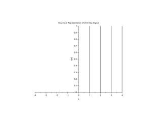
6. //Caption: Unit Step Sequence [Program]
clear;
clc;
close;
L = 4; //Upperlimit
n = -L:L;
x = [zeros(1,L),ones(1,L+1)];
a=gca();
a.y_location = "middle";
plot2d3('gnn',n,x)
title('Graphical Representation of Unit Step Signal')
xlabel(' n');
ylabel(' x[n]');

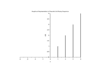
8. //Caption: Discrete Ramp Sequence [Program]
clear;
clc;
close;
L = 4; //Upperlimit
n = -L:L;
x = [zeros(1,L),0:L];
b = gca();
b.y_location = 'middle';
plot2d3('gnn',n,x)
a=gce();
a.children(1).thickness =2;
xtitle('Graphical Representation of Discrete Unit Ramp
Sequence','n','x[n]');

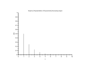
10. //Caption: Exponentially Decreasing Signal [Program]
clear;
clc;
close;
a =0.5;
n = 0:10;
x = (a)^n;
a=gca();
a.x_location = "origin";
a.y_location = "origin";
plot2d3('gnn',n,x)
a.thickness = 2;
xtitle('Graphical Representation of Exponentially Decreasing
Signal','n','x[n]');

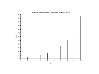
12. //Caption:Exponentially Increasing Signal [Program]
clear;
clc;
close;
a =1.5;
n =1:10;
x = (a)^n;
a=gca();
a.thickness = 2;
plot2d3('gnn',n,x)
xtitle('Graphical Representation of Exponentially
Increasing Signal','n','x[n]');

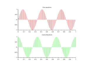
14. //Caption: Sine wave and Cosine wave plot [Program]
clc;
clear;
close;
f = 3; //Frequency = 3 Hertz
t = 0:0.01:1;
X = sin(2*%pi*f*t);
Y = cos(2*%pi*f*t);
subplot(2,1,1)
plot2d3('gnn',t,X,5)
title("Sine waveform")
subplot(2,1,2)
plot2d3('gnn',t,Y,3)
title('Cosine Waveform')

16. [2]. Linear Convolution
//Caption:Program for Linear Convolution [Program]
clc;
clear all;
close ;
x = input('enter x seq');
h = input('enter h seq');
m = length(x);
n = length(h);
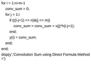
//Method 1 Using Direct Convolution Sum Formula

17. for i = 1:n+m-1
conv_sum = 0;
for j = 1:i
if (((i-j+1) <= n)&(j <= m))
conv_sum = conv_sum + x(j)*h(i-j+1);
end;
y(i) = conv_sum;
end;
end;
disp(y','Convolution Sum using Direct Formula Method
=')

18. //Method 2 Using Inbuilt Function
f = convol(x,h)
disp(f,'Convolution Sum Result using Inbuilt Funtion =')
subplot(3,1,1);
plot2d3('gnn',x)
xtitle('Graphical Representation of Input signal x');
subplot(3,1,2);
plot2d3('gnn',h)
xtitle('Graphical Representation of Impulse signal h');
subplot(3,1,3);
plot2d3('gnn',y)
xtitle('Graphical Representation of Output signal y');

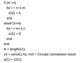
20. [3]. Circular Convolution
//Caption: Program to find the Cicrcular Convolution
of given [Program]
//discrete sequences using Matrix method
clear;
clc;
x1 = [2,1,2,1]; //First sequence
x2 = [1,2,3,4]; //Second sequence
m = length(x1); //length of first sequence
n = length(x2); //length of second sequence
//To make length of x1 and x2 are Equal

21. if (m >n)
for i = n+1:m
x2(i) = 0;
end
elseif (n>m)
for i = m+1:n
x1(i) = 0;
end
end
N = length(x1);
x3 = zeros(1,N); //x3 = Circular convolution result
a(1) = x2(1);

22. for j = 2:N
a(j) = x2(N-j+2);
end
for i =1:N
x3(1) = x3(1)+x1(i)*a(i);
end
X(1,:)=a;
//Calculation of circular convolution
for k = 2:N
for j =2:N
x2(j) = a(j-1);
end

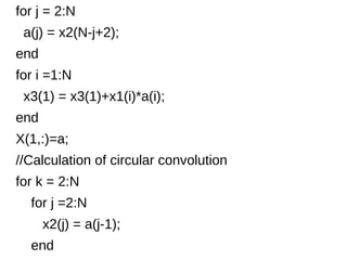
23. x2(1) = a(N);
X(k,:)= x2;
for i = 1:N
a(i) = x2(i);
x3(k) = x3(k)+x1(i)*a(i);
end
end
disp(X,'Circular Convolution Matrix x2[n]=')
disp(x3,'Circular Convolution Result x3[n] = ')
//Result
//Circular Convolution Matrix x2[n]=
// 1. 4. 3. 2.
// 2. 1. 4. 3.
// 3. 2. 1. 4.
// 4. 3. 2. 1.
// Circular Convolution Result x3[n] =
// 14. 16. 14. 16.

24. [4]. Linear Convolution using Circular Convolution
//Method 3 Linear Convolution using Circular Convolution
//Circular Convolution Using frequency Domain multiplication (DFT-IDFT method)
[Program]
N = n+m-1;
x = [x zeros(1,N-m)];
h = [h zeros(1,N-n)];
f1 = fft(x)
f2 = fft(h)
f3 = f1.*f2; // freq domain multiplication
f4 = ifft(f3)
disp(f4,'Convolution Sum Result DFT - IDFT method =')
//Result
//enter x seq [1 1 1 1]
//enter h seq [1 2 3]
// Convolution Sum Result DFT - IDFT method =
// 1. 3. 6. 6. 5. 3.

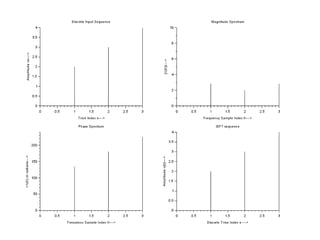
25. [5]. DFT and IDFT using Formula
//Caption: Discrete Fourier Transform and its Inverse
using formula
//Program to find the spectral information of discrete
time signal [Program]
clc;
close;
clear;
xn = input('Enter the real input discrete sequence
x[n]=');
N = length(xn);
XK = zeros(1,N);
IXK = zeros(1,N);

26. //Code block to find the DFT of the Sequence
for K = 0:N-1
for n = 0:N-1
XK(K+1) = XK(K+1)+xn(n+1)*exp(-%i*2*%pi*K*n/N);
end
end
[phase,db] = phasemag(XK)
disp(XK,'Discrete Fourier Transform X(k)=')
disp(abs(XK),'Magnitude Spectral Samples=')
disp(phase,'Phase Spectral Samples=')
n = 0:N-1;
K = 0:N-1;

27. subplot(2,2,1)
a = gca();
a.x_location = "origin";
a.y_location = "origin";
plot2d3('gnn',n,xn)
xlabel('Time Index n---->')
ylabel('Amplitude xn---->')
title('Discrete Input Sequence')
subplot(2,2,2)
a = gca();
a.x_location = "origin";
a.y_location = "origin";
plot2d3('gnn',K,abs(XK))

28. xlabel('Frequency Sample Index K---->')
ylabel('|X(K)|---->')
title('Magnitude Spectrum')
subplot(2,2,3)
a = gca();
a.x_location = "origin";
a.y_location = "origin";
plot2d3('gnn',K,phase)
xlabel('Frequency Sample Index K---->')
ylabel('<X(K) in radians---->')
title('Phase Spectrum')

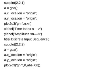
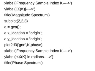
29. //Code block to find the IDFT of the sequence
for n = 0:N-1
for K = 0:N-1
IXK(n+1) = IXK(n+1)+XK(K+1)*exp(%i*2*%pi*K*n/N);
end
end
IXK = IXK/N;
ixn = real(IXK);
subplot(2,2,4)
a = gca();
a.x_location = "origin";
a.y_location = "origin";
plot2d3('gnn',[0:N-1],ixn)
xlabel('Discrete Time Index n ---->')
ylabel('Amplitude x[n]---->')
title('IDFT sequence')

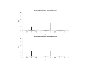
31. [6]. DFT and IDFT using FFT algorithm (inbuilt function)
//Caption:DFT and IDFT using FFT algorithm[Program]
clear;
clc;
close;
x = input("enter the input discrete sequence");
L = length(x); //Length of the Sequence
N = input('Enter the N-point value:='); // N -point DFT
//Computing DFT
X = fft(x,-1);
disp(X,'FFT of x[n] is X(k)=')
x =abs(fft(X,1))
disp(x,'IFFT of X(k) is x[n]=')

32. //Plotting the spectrum of Discrete Sequence
subplot(2,1,1)
a=gca();
a.data_bounds=[0,0;5,10];
plot2d3('gnn',0:length(x)-1,x)
b = gce();
b.children(1).thickness =3;
xtitle('Graphical Representation of Discrete Sequence','n','x[n]');
subplot(2,1,2)
a=gce();
a.data_bounds=[0,0;5,10];
plot2d3('gnn',0:length(X)-1,abs(X))
b = gce();
b.children(1).thickness =3;
xtitle('Graphical Representation of Discrete Spectrum','k','X(k)');

34. [7]. Discrete Cosine Transform and
Inverse Discrete Cosine Transform
Problem: If x[n] = {1,3,5,2,3,6,1,2} compute
signal in frequency domain using DCT
algorithm.
XDCT(K) = {8.131,-0.0342,-2.263,0.1573,-2.474,-
1.7718,2.8508,-0.5784}
xIDCT[n] = {1,3,5,2,3,6,1,2}
Program

35. //Caption: Discrete Cosine Transform and Inverse Discrete Cosine
Transform
clear;
clc;
close;
x = [1,3,5,2,3,6,1,2];
XDCT = dct(x,-1);//Discrete Cosine Transform
xIDCT = dct(XDCT,1);//Inverse Discrete Cosine Transform
disp(XDCT,'DCT of x[n]=')
disp(xIDCT,'Inverse DCT of x =')
//RESULT
//DCT of x[n]=
// 8.131728 - 0.0342533 - 2.2632715 0.1573526 - 2.4748737 -
1.7718504 2.8508949 - 0.5784576
// Inverse DCT of x =
// 1. 3. 5. 2. 3. 6. 1. 2.

36. [8]. Auto correlation and Cross correlation
a). Auto correlation [Program]
//Caption: Program to Compute the Autocorrelation of
a Sequence And verfication of Autocorrelation property
clc;
clear;
close;
x = input('Enter the input Sequence:=');
m = length(x);
lx = input('Enter the lower index of input sequence:=')
hx = lx+m-1;
n = lx:1:hx;

37. x_fold = x($:-1:1);
nx = lx+lx;
nh = nx+m+m-2;
r = nx:nh;
Rxx = convol(x,x_fold);
disp(Rxx,'Auto Correlation Rxx[n]:=')
//Property 1: Autocorrelation of a sequence has even symmetry
//Rxx[n] = Rxx[-n]
Rxx_flip = Rxx([$:-1:1]);
if Rxx_flip==Rxx then
disp('Property 1:Auto Correlation has Even Symmetry');
disp(Rxx_flip,'Auto Correlation time reversed Rxx[-n]:=');
end

38. //Property 2: Center value Rxx[0]= total power of the sequence
Tot_Px = sum(x.^2);
Mid = ceil(length(Rxx)/2);
if Tot_Px == Rxx(Mid) then
disp('Property 2:Rxx[0]=center value=max. value=Total power of i/p
sequence');
end
subplot(2,1,1)
plot2d3('gnn',n,x)
xlabel('n===>')
ylabel('Amplitude-->')
title('Input Sequence x[n]')
subplot(2,1,2)
plot2d3('gnn',r,Rxx)
xlabel('n===>')
ylabel('Amplitude-->')
title('Auto correlation Sequence Rxx[n]')

39. /Example
//Enter the input Sequence:=[2,-1,3,4,1]
//
//Enter the lower index of input sequence:=-2
//
// Auto Correlation Rxx[n]:=
//
// 2. 7. 5. 11. 31. 11. 5. 7. 2.
//
// Property 1:Auto Correlation has Even Symmetry
//
// Auto Correlation time reversed Rxx[-n]:=
//
// 2. 7. 5. 11. 31. 11. 5. 7. 2.
//
// Property 2:Rxx[0]=center value=max. value=Total power of i/p sequence

40. [b]. Cross Correlation [Program]

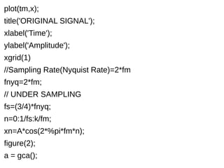
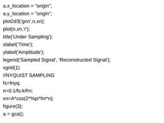
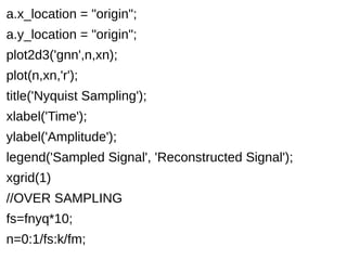
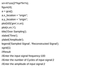
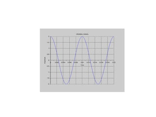
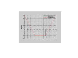
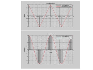
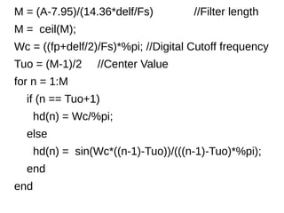
41. 9. Sampling and Aliasing Effect
//Caption: Verification of Sampling Theorem [Program]
//[1].Right Sampling [2]. Under Sampling [3]. Over Sampling
clc;
close;
clear;
fm=input('Enter the input signal frequency:');
k=input('Enter the number of Cycles of input signal:');
A=input('Enter the amplitude of input signal:');
tm=0:1/(fm*fm):k/fm;
x=A*cos(2*%pi*fm*tm);
figure(1);
a = gca();
a.x_location = "origin";
a.y_location = "origin";

42. plot(tm,x);
title('ORIGINAL SIGNAL');
xlabel('Time');
ylabel('Amplitude');
xgrid(1)
//Sampling Rate(Nyquist Rate)=2*fm
fnyq=2*fm;
// UNDER SAMPLING
fs=(3/4)*fnyq;
n=0:1/fs:k/fm;
xn=A*cos(2*%pi*fm*n);
figure(2);
a = gca();

43. a.x_location = "origin";
a.y_location = "origin";
plot2d3('gnn',n,xn);
plot(n,xn,'r');
title('Under Sampling');
xlabel('Time');
ylabel('Amplitude');
legend('Sampled Signal', 'Reconstructed Signal');
xgrid(1)
//NYQUIST SAMPLING
fs=fnyq;
n=0:1/fs:k/fm;
xn=A*cos(2*%pi*fm*n);
figure(3);
a = gca();

44. a.x_location = "origin";
a.y_location = "origin";
plot2d3('gnn',n,xn);
plot(n,xn,'r');
title('Nyquist Sampling');
xlabel('Time');
ylabel('Amplitude');
legend('Sampled Signal', 'Reconstructed Signal');
xgrid(1)
//OVER SAMPLING
fs=fnyq*10;
n=0:1/fs:k/fm;

45. xn=A*cos(2*%pi*fm*n);
figure(4);
a = gca();
a.x_location = "origin";
a.y_location = "origin";
plot2d3('gnn',n,xn);
plot(n,xn,'r');
title('Over Sampling');
xlabel('Time');
ylabel('Amplitude');
legend('Sampled Signal', 'Reconstructed Signal');
xgrid(1)
//Result
//Enter the input signal frequency:100
//Enter the number of Cycles of input signal:2
//Enter the amplitude of input signal:2

49. 10. FIR Digital Filter Design
Low Pass Filter Design [Program]
//Caption: Program to Design FIR Low Pass Filter
//Reference: Digital Signal Processing A Practical Approach
//by Emmaanuel Ifeachor and Barrie Jervis, Second
Edition, Pearson Education
clc;
close;
clear;
fp = input("Enter the passband edge frequency in Hz=")
delf = input("Enter the transition width in Hz =")
A = input("Enter the stop band attenuation in dB =")
Fs = input("Enter the sampling frequency in Hz=")

50. M = (A-7.95)/(14.36*delf/Fs) //Filter length
M = ceil(M);
Wc = ((fp+delf/2)/Fs)*%pi; //Digital Cutoff frequency
Tuo = (M-1)/2 //Center Value
for n = 1:M
if (n == Tuo+1)
hd(n) = Wc/%pi;
else
hd(n) = sin(Wc*((n-1)-Tuo))/(((n-1)-Tuo)*%pi);
end
end

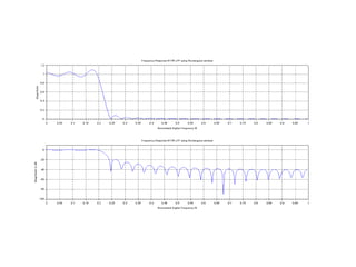
51. //Rectangular Window
for n = 1:M
W(n) = 1;
end
//Windowing Fitler Coefficients
h = hd.*W;
disp(h,'Filter Coefficients are')
[hzm,fr]=frmag(h,256);
hzm_dB = 20*log10(hzm)./max(hzm);
subplot(2,1,1)
plot(2*fr,hzm)
xlabel('Normalized Digital Frequency W');
ylabel('Magnitude');
title('Frequency Response 0f FIR LPF using Rectangular window')
xgrid(1)

52. subplot(2,1,2)
plot(2*fr,hzm_dB)
xlabel('Normalized Digital Frequency W');
ylabel('Magnitude in dB');
title('Frequency Response 0f FIR LPF using Rectangular
window')
xgrid(1)
//Result
///
//Enter the passband edge frequency in Hz=1500
//Enter the transition width in Hz =500
//Enter the stop band attenuation in dB =50
//Enter the sampling frequency in Hz=8000

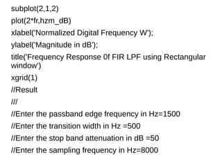
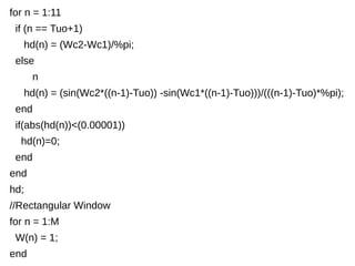
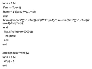
54. High Pass Filter Design [Program]
//Caption: Program to Design FIR High Pass Filter
clear;
clc;
close;
M = input('Enter the Odd Filter Length ='); //Filter length
Wc = input('Enter the Digital Cutoff frequency ='); //Digital Cutoff
frequency
Tuo = (M-1)/2 //Center Value
for n = 1:M
if (n == Tuo+1)
hd(n) = 1-Wc/%pi;
else
hd(n) = (sin(%pi*((n-1)-Tuo)) -sin(Wc*((n-1)-Tuo)))/(((n-1)-Tuo)*%pi);
end
end
//Rectangular Window
for n = 1:M
W(n) = 1;
end

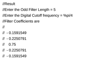
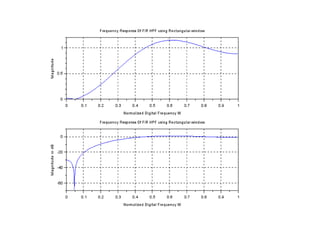
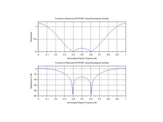
55. //Windowing Fitler Coefficients
h = hd.*W;
disp(h,'Filter Coefficients are')
[hzm,fr]=frmag(h,256);
hzm_dB = 20*log10(hzm)./max(hzm);
subplot(2,1,1)
plot(2*fr,hzm)
xlabel('Normalized Digital Frequency W');
ylabel('Magnitude');
title('Frequency Response 0f FIR HPF using Rectangular window')
xgrid(1)
subplot(2,1,2)
plot(2*fr,hzm_dB)
xlabel('Normalized Digital Frequency W');
ylabel('Magnitude in dB');
title('Frequency Response 0f FIR HPF using Rectangular window')
xgrid(1)

56. //Result
//Enter the Odd Filter Length = 5
//Enter the Digital Cutoff frequency = %pi/4
//Filter Coefficients are
//
// - 0.1591549
// - 0.2250791
// 0.75
// - 0.2250791
// - 0.1591549

58. Band Pass Filter [Program]
//Caption: Program to Design FIR Band Pass Filter
clear;
clc;
close;
M = input('Enter the Odd Filter Length ='); //Filter length
//Digital Cutoff frequency [Lower Cutoff, Upper Cutoff]
Wc = input('Enter the Digital Cutoff frequency =');
Wc2 = Wc(2)
Wc1 = Wc(1)
Tuo = (M-1)/2 //Center Value
hd = zeros(1,M);
W = zeros(1,M);

59. for n = 1:11
if (n == Tuo+1)
hd(n) = (Wc2-Wc1)/%pi;
else
n
hd(n) = (sin(Wc2*((n-1)-Tuo)) -sin(Wc1*((n-1)-Tuo)))/(((n-1)-Tuo)*%pi);
end
if(abs(hd(n))<(0.00001))
hd(n)=0;
end
end
hd;
//Rectangular Window
for n = 1:M
W(n) = 1;
end

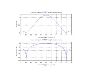
60. //Windowing Fitler Coefficients
h = hd.*W;
disp(h,'Filter Coefficients are')
[hzm,fr]=frmag(h,256);
hzm_dB = 20*log10(hzm)./max(hzm);
subplot(2,1,1)
plot(2*fr,hzm)
xlabel('Normalized Digital Frequency W');
ylabel('Magnitude');
title('Frequency Response 0f FIR BPF using Rectangular window')
xgrid(1)
subplot(2,1,2)
plot(2*fr,hzm_dB)
xlabel('Normalized Digital Frequency W');
ylabel('Magnitude in dB');
title('Frequency Response 0f FIR BPF using Rectangular window')
xgrid(1)

61. //Result
//Enter the Odd Filter Length = 11
//Enter the Digital Cutoff frequency = [%pi/4,3*%pi/4]
//Filter Coefficients are
// 0. 0. 0. - 0.3183099 0. 0.5 0. -
0.3183099 0. 0. 0.

63. FIR Band Stop Filter [Program]
//Caption: Program to Design FIR Band Reject Filter
clear ;
clc;
close;
M = input('Enter the Odd Filter Length ='); //Filter length
//Digital Cutoff frequency [Lower Cutoff, Upper Cutoff]
Wc = input('Enter the Digital Cutoff frequency =');
Wc2 = Wc(2)
Wc1 = Wc(1)
Tuo = (M-1)/2 //Center Value
hd = zeros(1,M);
W = zeros(1,M);

64. for n = 1:M
if (n == Tuo+1)
hd(n) = 1-((Wc2-Wc1)/%pi);
else
hd(n)=(sin(%pi*((n-1)-Tuo))-sin(Wc2*((n-1)-Tuo))+sin(Wc1*((n-1)-Tuo)))/
(((n-1)-Tuo)*%pi);
end
if(abs(hd(n))<(0.00001))
hd(n)=0;
end
end
//Rectangular Window
for n = 1:M
W(n) = 1;
end

65. //Windowing Fitler Coefficients
h = hd.*W;
disp(h,'Filter Coefficients are')
[hzm,fr]=frmag(h,256);
hzm_dB = 20*log10(hzm)./max(hzm);
subplot(2,1,1)
plot(2*fr,hzm)
xlabel('Normalized Digital Frequency W');
ylabel('Magnitude');
title('Frequency Response 0f FIR BSF using Rectangular window')
xgrid(1)
subplot(2,1,2)
plot(2*fr,hzm_dB)
xlabel('Normalized Digital Frequency W');
ylabel('Magnitude in dB');
title('Frequency Response 0f FIR BSF using Rectangular window')
xgrid(1)

67. [11]. IIR Butterworth Filter Design
(Digital Filter Design using Bilinear
Transform Method)
a) .Digital IIR Low Pass Butterworth Filter
b). Digital IIR High Pass Butterworth Filter
c). Digital IIR Band Pass Butterworth Filter
d).Digital IIR Band Stop Butterworth Filter

68. [12]. IIR Chebyshev Digital Filter
Design
(Using Bilinear Transformation)
Program

69. [13]. Power Spectrum Estimation
(Periodogram)
Program