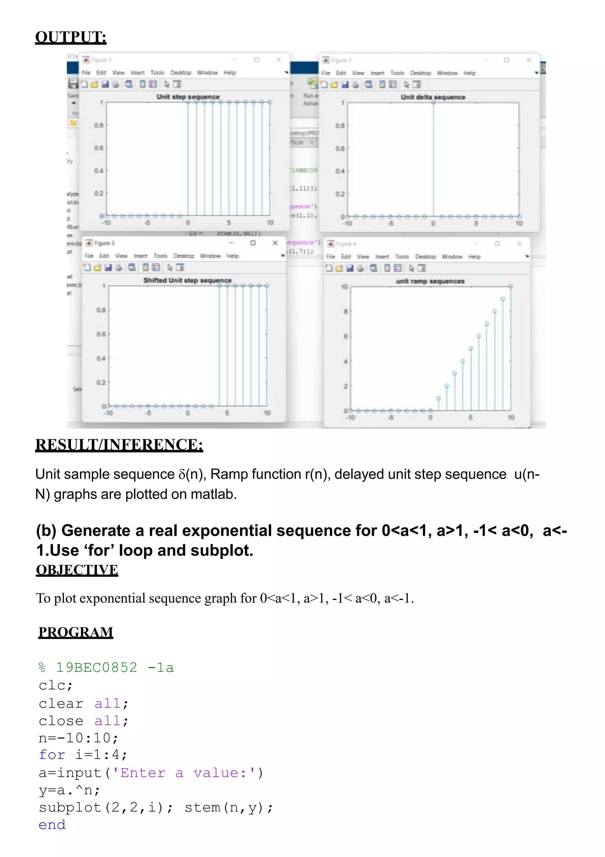
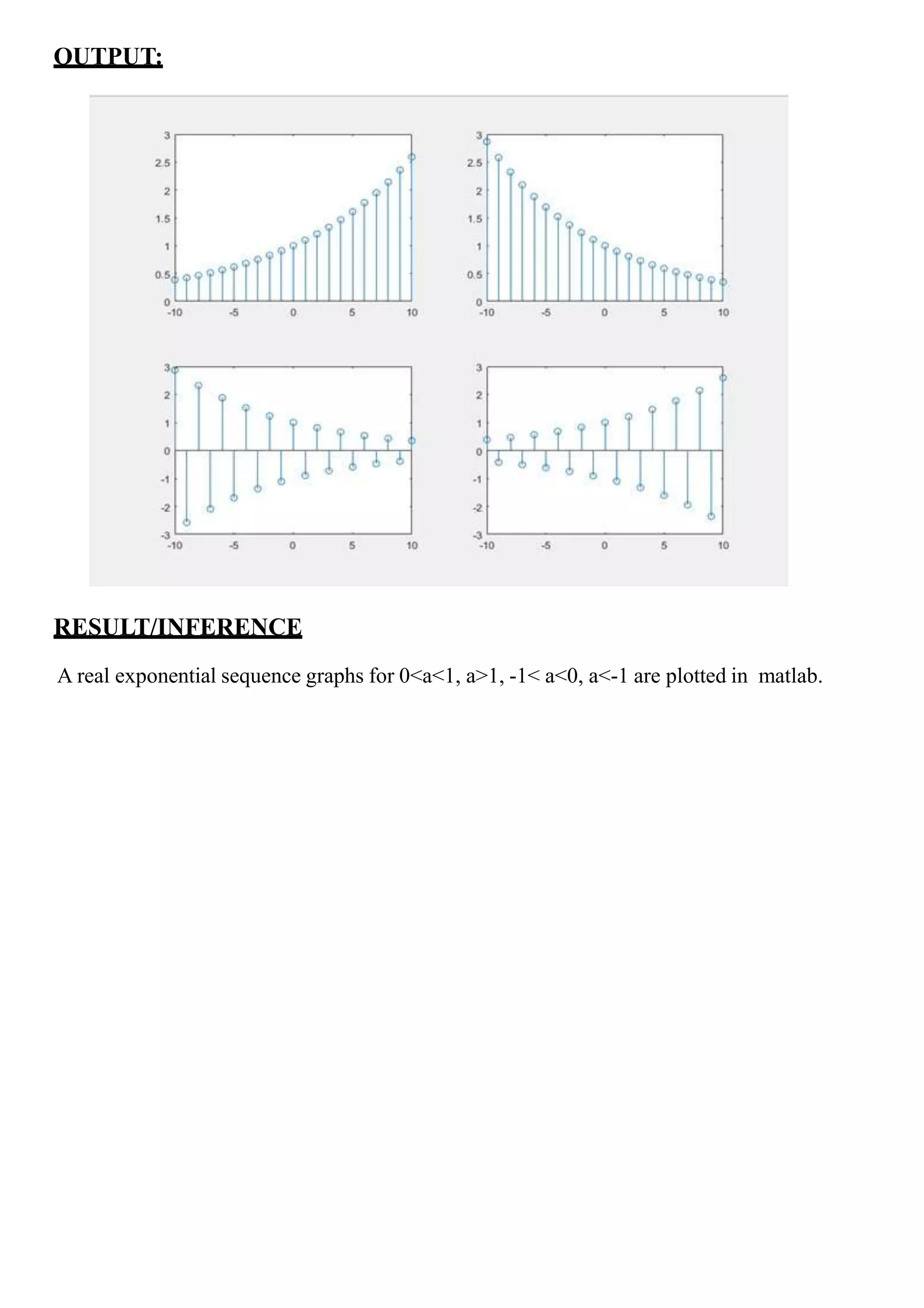
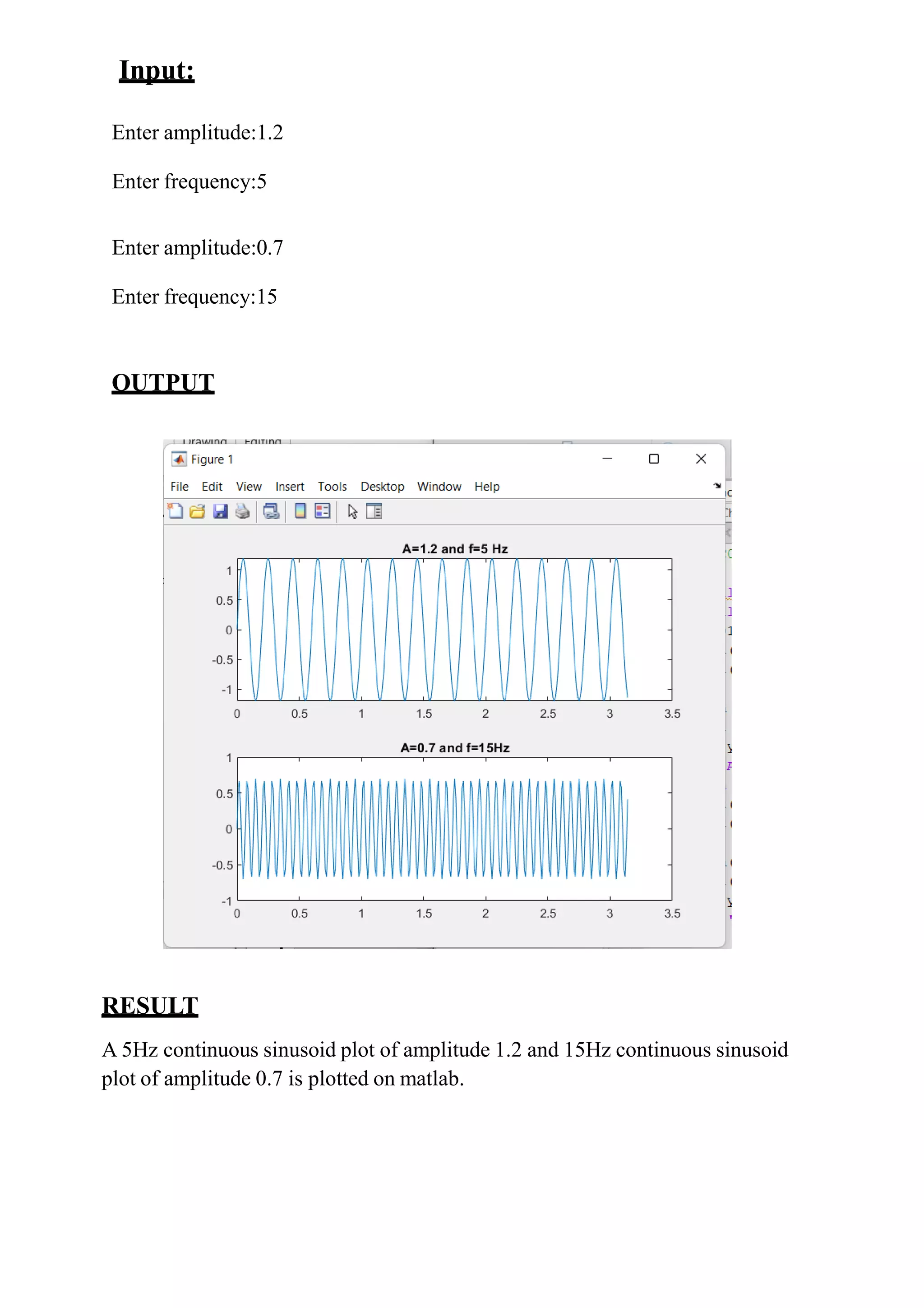
The document describes several MATLAB experiments involving digital signal processing tasks: 1. Plotting unit sample, step, delayed step, and ramp sequences. 2. Plotting exponential sequences for different values of a. 3. Plotting 5Hz and 15Hz sinusoidal signals with given amplitudes. 4. Plotting shifted unit step sequences and identifying them as causal, anti-causal, or non-causal. 5. Performing linear convolution of two sequences without using the conv function and verifying the result.

1. DIGITAL SIGNAL
PROCESSING
TASK-1
(a)
OBJECTIVE:
To generate unit sample sequence delta(n), unit step sequence u(n), delayed
unit step sequence u(n-N) where N=4, unit ramp sequence r(n).
PROGRAM:
% 19BEC0852 -1a
clc
clear all;
close all;
n=-10:1:10;
u=[zeros(1,10),ones(1,11)];
stem(n,u);
title('Unit step sequence')
del=[zeros(1,10),ones(1,1),zeros(
1,10)];
figure
stem(n,del);
title('Unit delta sequence')
u=[zeros(1,14),ones(1,7)];
figure
stem(n,u);
title('Shifted Unit step
sequence')
r=n.*(n>=0);
figure;
stem(n,r);
title('unit ramp sequences')
Name:- Naragam.Kiran Ganesh
Reg no:- 19BEC0852
Lab slot:L45+l46

2. OUTPUT:
RESULT/INFERENCE:
Unit sample sequence (n), Ramp function r(n), delayed unit step sequence u(n-
N) graphs are plotted on matlab.
(b) Generate a real exponential sequence for 0<a<1, a>1, -1< a<0, a<-
1.Use ‘for’ loop and subplot.
OBJECTIVE
To plot exponential sequence graph for 0<a<1, a>1, -1< a<0, a<-1.
PROGRAM
% 19BEC0852 -1a
clc;
clear all;
close all;
n=-10:10;
for i=1:4;
a=input('Enter a value:')
y=a.^n;
subplot(2,2,i); stem(n,y);
end

3. OUTPUT:
RESULT/INFERENCE
A real exponential sequence graphs for 0<a<1, a>1, -1< a<0, a<-1 are plotted in matlab.

4. (c) Generate a 5Hz continuous sinusoid plot of amplitude
1.2 and 15Hz continuous sinusoid plot of amplitude 0.7. Comment
on the sampling frequency.
OBJECTIVE:
To generate a 5Hz continuous sinusoid plot of amplitude 1.2 and 15Hz
continuous sinusoid plot of amplitude 0.7 .
PROGRAM:
% 19BEC0852 -1c
clc
clear all
close all
t=0:0.01:pi;
a=input('Enter amplitude:');
f=input('Enter frequency:');
T=1/f;
y=a*sin (2*pi*f*t);
subplot (2,1,1);
plot(t,y)
title('A=1.2 and f=5 Hz')
hold on
a=input('Enter amplitude:');
f=input('Enter frequency:');
T=1/f;
y=a*sin(2*pi*f*t);
subplot(2,1,2);
plot(t,y)
title ('A=0.7 and f=15Hz')

5. Input:
Enter amplitude:1.2
Enter frequency:5
Enter amplitude:0.7
Enter frequency:15
OUTPUT
RESULT
A 5Hz continuous sinusoid plot of amplitude 1.2 and 15Hz continuous sinusoid
plot of amplitude 0.7 is plotted on matlab.

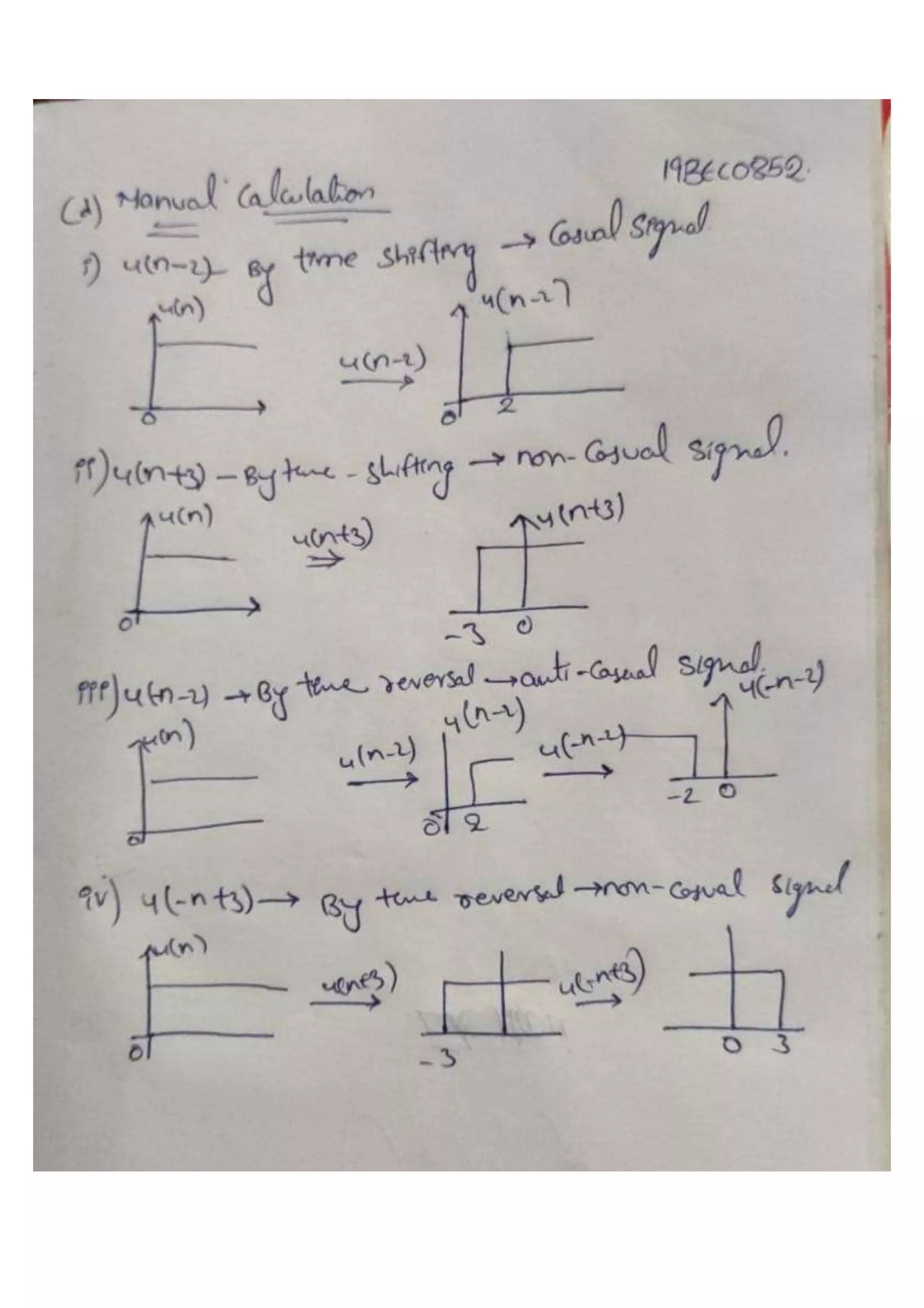
6. (d) Plot 𝑢(𝑛− 2), 𝑢(𝑛+ 3), 𝑢(−𝑛− 2), 𝑢(−𝑛+ 3) from -10 to 10 time
indices. Indicate which signal is causal, anti-causal and non-
causal.
OBJECTIVE
To plot (𝑛− 2),𝑢(𝑛+ 3),𝑢(−𝑛− 2),𝑢(−𝑛+ 3) from -10 to 10 time indices and to
check whether it is causal, anti-causal and non-causal.
% 19BEC0852-1d
clc;
clear all;
close all;
n=-10:10;
u1=[zeros(1,12),ones(1,9)];
u2=[zeros(1,7),ones(1,14)];
u3=[ones(1,9),zeros(1,12)];
u4=[ones(1,14),zeros(1,7)];
subplot(2,2,1);
stem(n,u1);
subplot(2,2,2);
stem(n,u2);
subplot(2,2,3);
stem(n,u3);
subplot(2,2,4);
stem(n,u4);
PROGRAM:
OUTPUT

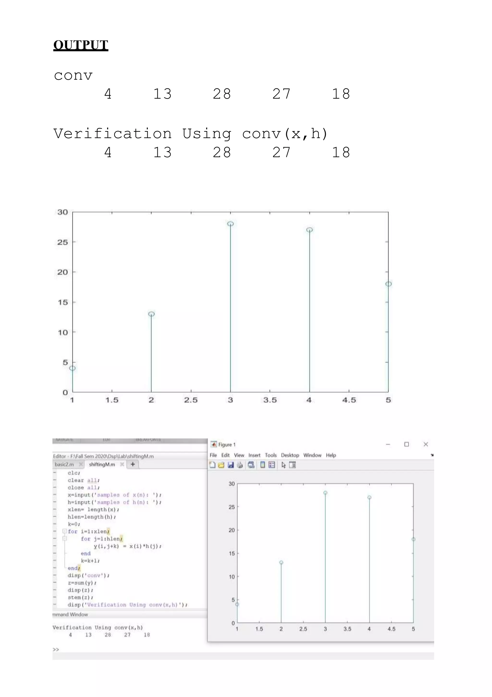
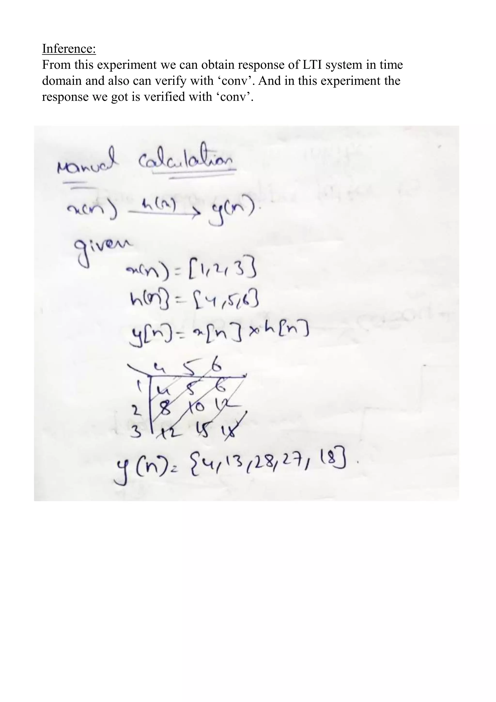
8. 2. Using MATLAB perform the linear convolution between input
x(n) and impulse response h(n) to obtain the response of LTI
system y(n) in the time domain without using the inbuilt function
‘conv’. Verify the result using ‘conv’.
OBJECTIVE
Using matlab perform the linear convolution b/w input x(n) and impulse
response h(n).
PROGRAM
clc;
clear all;
close all;
x=input('samples of x(n): ');
h=input('samples of h(n): ');
xlen= length(x);
hlen=length(h);
k=0;
for i=1:xlen;
for j=1:hlen;
y(i,j+k) = x(i)*h(j);
end
k=k+1;
end;
disp('conv');
z=sum(y);
disp(z);
stem(z);
disp('Verification Using conv(x,h)');
disp(conv(x,h));
INPUT
samples of x(n): [1 2 3]
samples of h(n): [4 5 6]

9. OUTPUT
conv
4 13 28 27 18
Verification Using conv(x,h)
4 13 28 27 18

10. Inference:
From this experiment we can obtain response of LTI system in time
domain and also can verify with ‘conv’. And in this experiment the
response we got is verified with ‘conv’.