The document is a lab manual for basic simulation experiments. It contains 18 listed experiments related to signals and systems including: basic operations on matrices, generation of periodic and aperiodic signals, arithmetic operations on signals, finding even and odd parts of signals, linear convolution, autocorrelation and cross correlation. The document provides brief descriptions and MATLAB code examples for experiments related to signals and systems analysis.


![BASIC OPERATIONS ON MATRICES
Aim: To generate matrix and perform basic operation on matrices Using
MATLAB Software.
EQUIPMENTS:
PC with windows (95/98/XP/NT/2000).
MATLAB Software
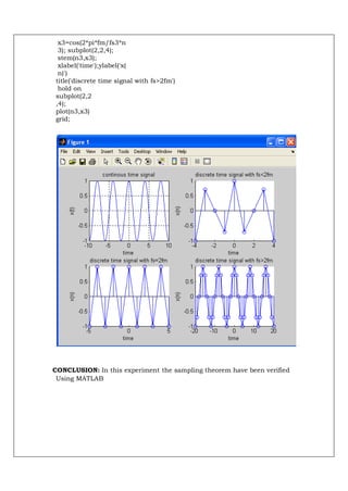
CONCLUSION:
EXP.NO: 2
GENERATION OF VARIOUS SIGNALS AND SEQUENCES (PERIODIC
AND APERIODIC), SUCH AS UNIT IMPULSE, UNIT STEP,
SQUARE, SAWTOOTH, TRIANGULAR, SINUSOIDAL, RAMP,
SINC.
Aim: To generate different types of signals Using MATLAB Software.
EQUIPMENTS:
PC with windows
(95/98/XP/NT/2000).
MATLAB Software
Matlab program:
%unit impulse
generation clc
close all
n1=-3;
n2=4;
n0=0;
n=[n1:n
2];
x=[(n-n0)==0]
stem(n,x)
% unit step
generation n1=-4;
n2=5;
n0=0;](https://image.slidesharecdn.com/basicsimulationlabmanual1-120709021807-phpapp01/85/Basic-simulation-lab-manual1-4-320.jpg)

![[y,n]=stepseq(n0,n1,n2);
stem(n,y); xlabel('n') ylabel('amplitude'); title('unit step');](https://image.slidesharecdn.com/basicsimulationlabmanual1-120709021807-phpapp01/85/Basic-simulation-lab-manual1-6-320.jpg)
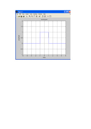
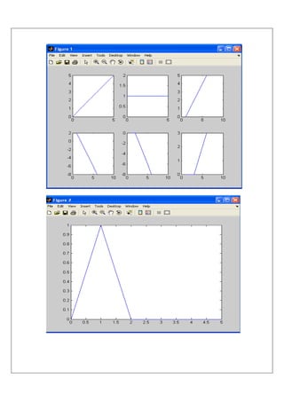
![% square wave wave
generator fs = 1000;
t = 0:1/fs:1.5;
x1 = sawtooth(2*pi*50*t); x2 =
square(2*pi*50*t);
subplot(2,2,1),plot(t,x1), axis([0 0.2 -1.2
1.2])
xlabel('Time (sec)');ylabel('Amplitude'); title('Sawtooth Periodic Wave')
subplot(2,2,2),plot(t,x2), axis([0 0.2 -1.2 1.2])
xlabel('Time (sec)');ylabel('Amplitude'); title('Square Periodic Wave');
subplot(2,2,3),stem(t,x2), axis([0 0.1 -1.2 1.2])
xlabel('Time (sec)');ylabel('Amplitude');
% sawtooth wave
generator fs = 10000;
t = 0:1/fs:1.5;
x = sawtooth(2*pi*50*t);
subplot(1,2,1);
plot(t,x), axis([0 0.2 -1
1]);
xlabel('t'),ylabel('x(t)')
title('sawtooth signal');
N=2; fs = 500;n =
0:1/fs:2; x =
sawtooth(2*pi*50*n);
subplot(1,2,2);](https://image.slidesharecdn.com/basicsimulationlabmanual1-120709021807-phpapp01/85/Basic-simulation-lab-manual1-7-320.jpg)
![stem(n,x), axis([0 0.2 -1
1]);
xlabel('n'),ylabel('x(n)')
title('sawtooth
sequence');
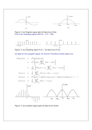
To generate a trianguular pulse
A=2; t = 0:0.0005:1;
x=A*sawtooth(2*pi*5*t,0.25); %5 Hertz wave with duty cycle 25%
plot(t,x);
grid
axis([0 1 -3 3]);
%%To generate a trianguular
pulse fs = 10000;t = -1:1/fs:1;
x1 = tripuls(t,20e-3); x2 = rectpuls(t,20e-3);
subplot(211),plot(t,x1), axis([-0.1 0.1 -0.2 1.2])
xlabel('Time (sec)');ylabel('Amplitude'); title('Triangular Aperiodic Pulse')
subplot(212),plot(t,x2), axis([-0.1 0.1 -0.2 1.2])](https://image.slidesharecdn.com/basicsimulationlabmanual1-120709021807-phpapp01/85/Basic-simulation-lab-manual1-8-320.jpg)
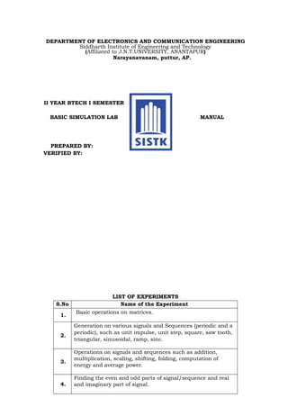
![xlabel('Time (sec)');ylabel('Amplitude'); title('Rectangular Aperiodic Pulse')
set(gcf,'Color',[1 1 1]),
%%To generate a rectangular pulse
t=-5:0.01:5;
pulse = rectpuls(t,2); %pulse of width 2 time units
plot(t,pulse)
axis([-5 5 -1 2]);
grid](https://image.slidesharecdn.com/basicsimulationlabmanual1-120709021807-phpapp01/85/Basic-simulation-lab-manual1-9-320.jpg)
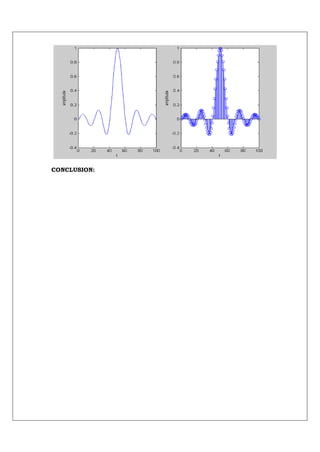
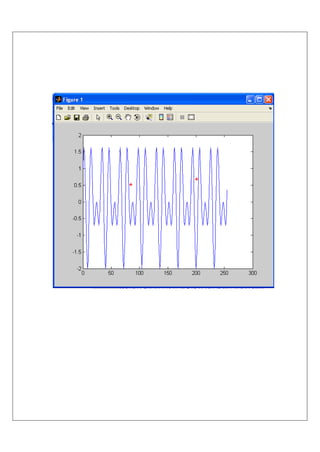
![% sinusoidal signal
N=64; % Define Number of samples
n=0:N-1; % Define vector
n=0,1,2,3,...62,63 f=1000; % Define
the frequency
fs=8000; % Define the sampling
frequency x=sin(2*pi*(f/fs)*n); %
Generate x(t) plot(n,x); % Plot x(t) vs.
t
title('Sinewave [f=1KHz,
fs=8KHz]'); xlabel('Sample
Number'); ylabel('Amplitude');
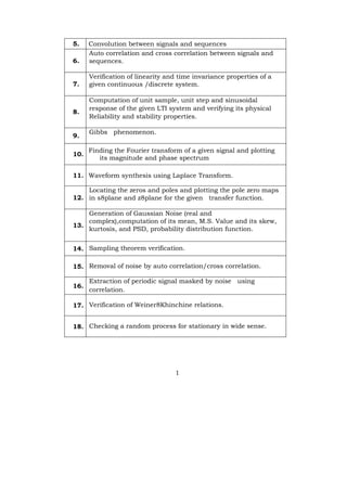
% RAMP
clc
close all
n=input('enter the length of ramp');
t=0:n; plot(t); xlabel('t');](https://image.slidesharecdn.com/basicsimulationlabmanual1-120709021807-phpapp01/85/Basic-simulation-lab-manual1-11-320.jpg)

![EXP.NO: 3
OPERATIONS ON SIGNALS AND SEQUENCES SUCH AS ADDITION,
MULTIPLICATION, SCALING, SHIFTING, FOLDING,
COMPUTATION OF ENERGY AND AVERAGE POWER
Aim: To perform arithmetic operations different types of signals Using
MATLAB Software.
EQUIPMENTS:
PC with windows
(95/98/XP/NT/2000).
MATLAB Softwar
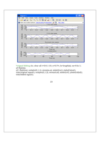
%plot the 2 Hz sine wave in the top panel
t = [0:.01:1]; % independent (time) variable
A = 8; % amplitude
f1 = 2; % create a 2 Hz sine wave lasting
1 sec s1 = A*sin(2*pi*f1*t);
f2 = 6; % create a 4 Hz sine wave lasting
1 sec s2 = A*sin(2*pi*f2*t);
figure subplot(4,1,1) plot(t, s1)
title('1 Hz sine wave')
ylabel('Amplitude')
%plot the 4 Hz sine wave in the middle panel subplot(4,1,2)
plot(t, s2)
title('2 Hz sine wave')
ylabel('Amplitude')
%plot the summed sine waves in the bottom panel subplot(4,1,3)
plot(t, s1+s2) title('Summed sine waves') ylabel('Amplitude') xlabel('Time (s)')
xmult=s1.*s2;
subplot(4,1,4); plot(xmult); title('multiplication'); ylabel('Amplitude') xlabel('Time (s)')](https://image.slidesharecdn.com/basicsimulationlabmanual1-120709021807-phpapp01/85/Basic-simulation-lab-manual1-16-320.jpg)
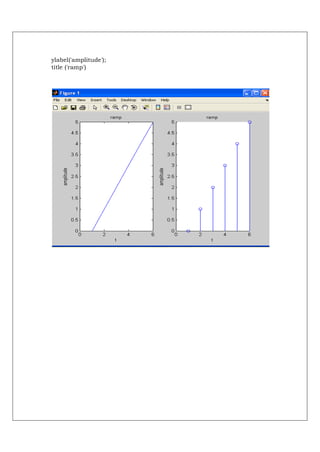
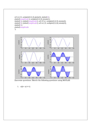
![%plot the 2 Hz sine wave scalling
t = [0:.01:1]; % independent (time) variable
A = 8; % amplitude
f1 = 2; % create a 2 Hz sine wave
lasting 1 sec s1 = A*sin(2*pi*f1*t);
subplot(3,2,1) plot(s1); xlabel('t');
ylabel('amplitude'); s2=2*s1; subplot(3,2,2) plot(s2);
xlabel('t');
ylabel('amplitude');](https://image.slidesharecdn.com/basicsimulationlabmanual1-120709021807-phpapp01/85/Basic-simulation-lab-manual1-18-320.jpg)
![EXP.NO: 4
FINDING THE EVEN AND ODD PARTS OF SIGNAL/SEQUENCE AND
REAL AND IMAGINARY PART OF SIGNAL
Aim: program for finding even and odd parts of signals Using MATLAB
Software.
EQUIPMENTS:
PC with windows
(95/98/XP/NT/2000). MATLAB
Software
%even and odd signals program:
t=-4:1:4;
h=[ 2 1 1 2 0 1 2 2 3 ];
subplot(3,2,1)
stem(t,h);
xlabel('time'); ylabel('amplitude');
title('signal');
n=9;](https://image.slidesharecdn.com/basicsimulationlabmanual1-120709021807-phpapp01/85/Basic-simulation-lab-manual1-21-320.jpg)
![% energy clc;
close all; clear all; x=[1,2,3]; n=3
e=0;
for i=1:n;
e=e+(x(i).*x(i));
end
% energy clc;
close all; clear all; N=2 x=ones(1,N) for i=1:N
y(i)=(1/3)^i.*x(i);
end n=N;
e=0;
for i=1:n;
e=e+(y(i).*y(i));
end](https://image.slidesharecdn.com/basicsimulationlabmanual1-120709021807-phpapp01/85/Basic-simulation-lab-manual1-23-320.jpg)
![%
power
clc;
close all;
clear all;
N=2
x=ones(1,
N) for
i=1:N
y(i)=(1/3)^i.*x(i);
end
n=
N;
e=0
;
for i=1:n;
e=e+(y(i).*y(i))
;
end
p=e/(2*N+
1);
% power
N=input('type a value for
N'); t=-N:0.0001:N;
x=cos(2*pi*50*t).^2;
disp('the calculated power p of the
signal is'); P=sum(abs(x).^2)/length(x)
plot(t,x);
axis([0 0.1 0 1]);
disp('the theoretical power of the
signal is'); P_theory=3/8
CONCLUSION:](https://image.slidesharecdn.com/basicsimulationlabmanual1-120709021807-phpapp01/85/Basic-simulation-lab-manual1-24-320.jpg)
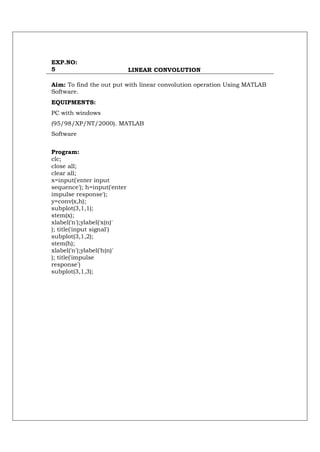
![stem(y);
xlabel('n');ylabel('y(n)')
; title('linear
convolution')
disp('The resultant signal is');
disp(y)
linear convolution
output:
enter input sequence[1 4 3
2] enter impulse response[1
0 2 1] The resultant signal
is
1 4 5 11 10 7 2](https://image.slidesharecdn.com/basicsimulationlabmanual1-120709021807-phpapp01/85/Basic-simulation-lab-manual1-26-320.jpg)

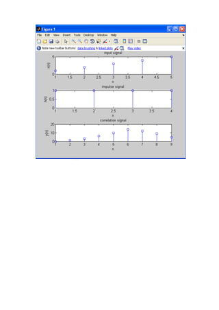
![% auto
correlation clc;
close all;
clear all;
x = [1,2,3,4,5]; y = [4,1,5,2,6];
subplot(3,1,
1); stem(x);
xlabel('n');
ylabel('x(n)');
title('input
signal');
subplot(3,1,2);
stem(y);
xlabel('n');
ylabel('y(n)');
title('input
signal');
z=xcorr(x,x);
subplot(3,1,3);
stem(z);
xlabel('n');
ylabel('z(n)');
title('resultant signal signal');](https://image.slidesharecdn.com/basicsimulationlabmanual1-120709021807-phpapp01/85/Basic-simulation-lab-manual1-30-320.jpg)
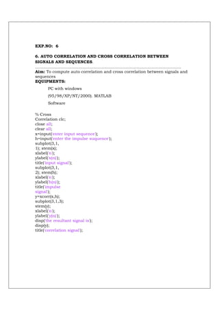
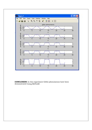
![CONCLUSION: In this experiment correlation of various signals
have been performed Using MATLAB
Applications:it is used to measure the degree to which the two signals are
similar and it is also used for radar detection by estimating the time delay.it
is also used in Digital communication, defence applications and sound
navigation
Excersize questions: perform convolution between the following signals
1. X(n)=[1 -1 4 ], h(n) = [ -1 2 -3 1]
2. perform convolution between the. Two periodic
sequences x1(t)=e-3t{u(t)-u(t-2)} , x2(t)= e -3t
for 0 ≤ t ≤ 2](https://image.slidesharecdn.com/basicsimulationlabmanual1-120709021807-phpapp01/85/Basic-simulation-lab-manual1-31-320.jpg)
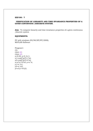
![D=10
;
x=3*cos(2*pi*0.1*n)-2*cos(2*pi*0.4*n);
xd=[zeros(1,D)
x];
y=n.*xd(n+D);
n1=n+D;
yd=n1.*x;
d=y-yd;
if d
disp('Given system is not satisfy time shifting property');
else
disp('Given system is satisfy time shifting property');
end
subplot(3,1,1),stem(y),gri
d;
subplot(3,1,2),stem(yd),g
rid;
subplot(3,1,3),stem(d),gri
d;](https://image.slidesharecdn.com/basicsimulationlabmanual1-120709021807-phpapp01/85/Basic-simulation-lab-manual1-36-320.jpg)
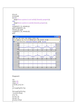
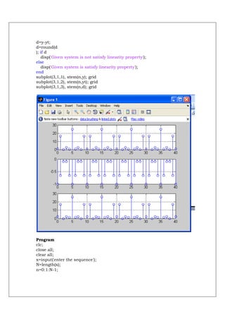
![Program
2:
clc;
close
all;
clear
all;
n=0:40;
D=10;
x=3*cos(2*pi*0.1*n)-2*cos(2*pi*0.4*n);
xd=[zeros(1,D)
x]; x1=xd(n+D);
y=exp(x1);
n1=n+D;
yd=exp(xd(n1));
d=y-yd;
if d
disp('Given system is not satisfy time shifting property');
else
disp('Given system is satisfy time shifting property');
end
subplot(3,1,1),stem(y),gri
d;
subplot(3,1,2),stem(yd),g
rid;
subplot(3,1,3),stem(d),gri
d;](https://image.slidesharecdn.com/basicsimulationlabmanual1-120709021807-phpapp01/85/Basic-simulation-lab-manual1-37-320.jpg)
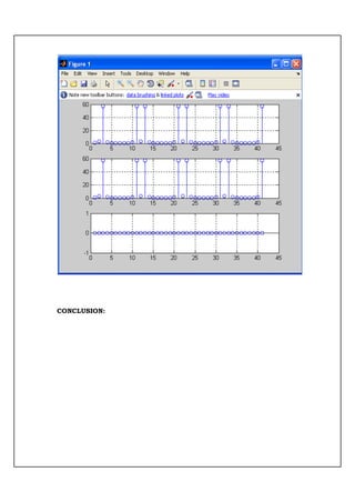
![EXP.NO:8
COMPUTATION OF UNIT SAMPLE, UNIT STEP AND SINUSOIDAL
RESPONSE OF THE GIVEN LTI SYSTEM AND VERIFYING ITS
PHYSICAL REALIZABILITY AND STABILITY PROPERTIES.
Aim: To Unit Step And Sinusoidal Response Of The Given LTI System And
Verifying
Its Physical Realizability And Stability
Properties.
EQUIPMENTS:
PC with windows
(95/98/XP/NT/2000).
MATLAB
Software
%calculate and plot the impulse response and step
response b=[1];
a=[1,-1,.9];
x=impseq(0,-20,120); n = [-20:120]; h=filter(b,a,x); subplot(3,1,1);stem(n,h);
title('impulse response'); xlabel('n');ylabel('h(n)');
=stepseq(0,-20,120); s=filter(b,a,x); s=filter(b,a,x); subplot(3,1,2); stem(n,s);
title('step response'); xlabel('n');ylabel('s(n)') t=0:0.1:2*pi;
x1=sin(t);
%impseq(0,-20,120); n = [-20:120]; h=filter(b,a,x1); subplot(3,1,3);stem(h);
title('sin response'); xlabel('n');ylabel('h(n)'); figure;
zplane(b,a);](https://image.slidesharecdn.com/basicsimulationlabmanual1-120709021807-phpapp01/85/Basic-simulation-lab-manual1-39-320.jpg)
![MATLAB Software
Program:
clc;
close all;
clear all;
x=input('enter the sequence'); N=length(x);
n=0:1:N-1; y=fft(x,N) subplot(2,1,1); stem(n,x);
title('input sequence'); xlabel('time index n----->'); ylabel('amplitude x[n]-
---> '); subplot(2,1,2);
stem(n,y);
title('output sequence');
xlabel(' Frequency index K---->');
ylabel('amplitude X[k]------>');](https://image.slidesharecdn.com/basicsimulationlabmanual1-120709021807-phpapp01/85/Basic-simulation-lab-manual1-45-320.jpg)
![FFT magnitude and Phase plot:
clc
close all x=[1,1,1,1,zeros(1,4)]; N=8;
X=fft(x,N); magX=abs(X),phase=angle(X)*180/pi; subplot(2,1,1)
plot(magX); grid xlabel('k')
ylabel('X(K)') subplot(2,1,2) plot(phase);](https://image.slidesharecdn.com/basicsimulationlabmanual1-120709021807-phpapp01/85/Basic-simulation-lab-manual1-46-320.jpg)


![Signal synthese using Laplace Tnasform:
clear all clc t=0:1:5 s=(t);
subplot(2,3,1) plot(t,s); u=ones(1,6) subplot(2,3,2) plot(t,u); f1=t.*u;
subplot(2,3,3) plot(f1);
s2=-2*(t-1); subplot(2,3,4); plot(s2);
u1=[0 1 1 1 1 1]; f2=-2*(t-1).*u1; subplot(2,3,5); plot(f2);
u2=[0 0 1 1 1 1]; f3=(t-2).*u2; subplot(2,3,6); plot(f3); f=f1+f2+f3; figure;
plot(t,f);
% n=exp(-t);
% n=uint8(n);
% f=uint8(f);
% R = int(f,n,0,6)
laplace(f);](https://image.slidesharecdn.com/basicsimulationlabmanual1-120709021807-phpapp01/85/Basic-simulation-lab-manual1-50-320.jpg)

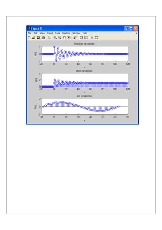
![EXP.NO: 12
LOCATING THE ZEROS AND POLES AND PLOTTING THE POLE ZERO
MAPS IN S-PLANE AND Z-PLANE FOR THE GIVEN TRANSFER FUNCTION.
Aim: To locating the zeros and poles and plotting the pole zero maps in
s-plane and z- plane for the given transfer function
EQUIPMENTS:
PC with windows (95/98/XP/NT/2000).
MATLAB Software
clc; close all clear all;
%b= input('enter the numarator cofficients')
%a= input('enter the denumi cofficients')
b=[1 2 3 4] a=[1 2 1 1 ] zplane(b,a);
Result: :](https://image.slidesharecdn.com/basicsimulationlabmanual1-120709021807-phpapp01/85/Basic-simulation-lab-manual1-53-320.jpg)
![EXP.NO: 13
13. Gaussian noise
%Estimation of Gaussian density and Distribution Functions
%% Closing and Clearing
all clc;
clear all;
close all;
%% Defining the range for the Random
variable dx=0.01; %delta x
x=-3:dx:3; [m,n]=size(x);
%% Defining the parameters of the pdf
mu_x=0; % mu_x=input('Enter the value of mean');
sig_x=0.1; % sig_x=input('Enter the value of varience');
%% Computing the probability density
function px1=[];
a=1/(sqrt(2*pi)*sig_x);
for j=1:n
px1(j)=a*exp([-((x(j)-mu_x)/sig_x)^2]/2);
end
%% Computing the cumulative distribution
function cum_Px(1)=0;
for j=2:n
cum_Px(j)=cum_Px(j-1)+dx*px1(j);
end
%% Plotting the
results figure(1)
plot(x,px1);grid
axis([-3 3 0 1]);
title(['Gaussian pdf for mu_x=0 and sigma_x=', num2str(sig_x)]);
xlabel('--> x')
ylabel('--> pdf')
figure(2)
plot(x,cum_Px);gri
d axis([-3 3 0 1]);
title(['Gaussian Probability Distribution Function for mu_x=0 and
sigma_x=', num2str(sig_x)]);
title('ite^{omegatau} = cos(omegatau) + isin(omegatau)')
xlabel('--> x')
ylabel('--> PDF')](https://image.slidesharecdn.com/basicsimulationlabmanual1-120709021807-phpapp01/85/Basic-simulation-lab-manual1-54-320.jpg)


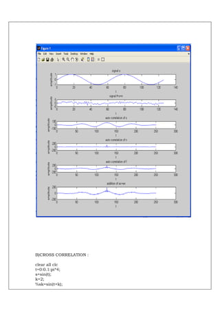
![REMOVAL OF NOISE BY AUTO CORRELATION/CROSS
CORRELATION
Aim: removal of noise by auto correlation/cross correlation
EQUIPMENTS:
PC with windows (95/98/XP/NT/2000).
MATLAB Software
a)auto correlation clear all
clc t=0:0.1:pi*4; s=sin(t);
k=2; subplot(6,1,1) plot(s); title('signal s'); xlabel('t');
ylabel('amplitude'); n = randn([1 126]); f=s+n; subplot(6,1,2) plot(f);
title('signal f=s+n'); xlabel('t'); ylabel('amplitude'); as=xcorr(s,s); subplot(6,1,3)
plot(as);
title('auto correlation of s'); xlabel('t'); ylabel('amplitude'); an=xcorr(n,n);
subplot(6,1,4)
plot(an);
title('auto correlation of
n'); xlabel('t');
ylabel('amplitude');
cff=xcorr(f,f);
subplot(6,1,5)
plot(cff);
title('auto correlation of
f'); xlabel('t');
ylabel('amplitude');
hh=as+an;
subplot(6,1,6)
plot(hh);
title('addition of
as+an'); xlabel('t');
ylabel('amplitude');](https://image.slidesharecdn.com/basicsimulationlabmanual1-120709021807-phpapp01/85/Basic-simulation-lab-manual1-63-320.jpg)
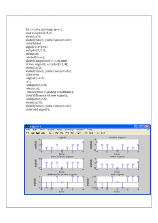
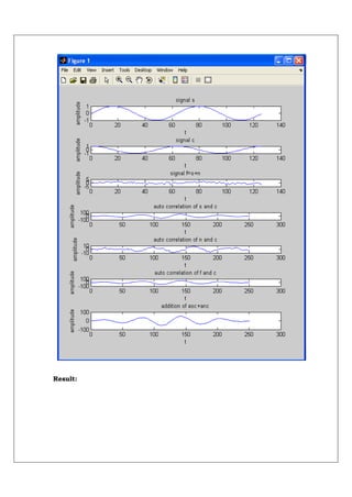
![subplot(7,1,1)
plot(s);
title('signal s');xlabel('t');ylabel('amplitude');
c=cos(t); subplot(7,1,2) plot(c);
title('signal c');xlabel('t');ylabel('amplitude');
n = randn([1 126]); f=s+n; subplot(7,1,3) plot(f);
title('signal f=s+n');xlabel('t');ylabel('amplitude');
asc=xcorr(s,c); subplot(7,1,4) plot(asc);
title('auto correlation of s and c');xlabel('t');ylabel('amplitude');
anc=xcorr(n,c); subplot(7,1,5) plot(anc);
title('auto correlation of n and c');xlabel('t');ylabel('amplitude');
cfc=xcorr(f,c); subplot(7,1,6) plot(cfc);
title('auto correlation of f and c');xlabel('t');ylabel('amplitude');
hh=asc+anc; subplot(7,1,7) plot(hh);
title('addition of asc+anc');xlabel('t');ylabel('amplitude');
76](https://image.slidesharecdn.com/basicsimulationlabmanual1-120709021807-phpapp01/85/Basic-simulation-lab-manual1-65-320.jpg)

![EXP.No:16
Program:
EXTRACTION OF
Clear all; close all; clc; n=256; k1=0:n-1;
P
x=cos(32*pi*k1/n)+sin(48*pi*k1/n);
E
plot(k1,x)
R
%Module to find period of input signl k=2;
I
xm=zeros(k,1); ym=zeros(k,1); hold on
O
for i=1:k
D
[xm(i) ym(i)]=ginput(1);
I
plot(xm(i), ym(i),'r*');
C
end
period=abs(xm(2)-xm(1)); rounded_p=round(period);
S
m=rounded_p
I
% Adding noise and plotting noisy signal
G
N
A
L
M
A
y=x+randn(1,n);
S
figure plot(k1,y)
K
E
D
B
Y
N
O
I
S
E
U
S
I
N
G
C
O
R
R
E
L
A
T
I
O
N
Extraction of
Periodic Signal
Masked By Noise
Using
Correlation](https://image.slidesharecdn.com/basicsimulationlabmanual1-120709021807-phpapp01/85/Basic-simulation-lab-manual1-68-320.jpg)

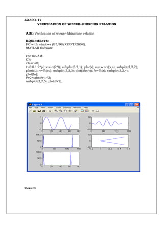
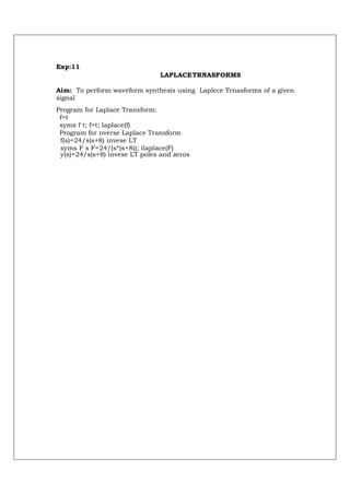
![EXP18.
CHECKING A RANDOM PROCESS FOR STATIONARITY IN WIDE SENSE.
AIM: Checking a random process for stationary in wide sense.
EQUIPMENTS:
PC with windows (95/98/XP/NT/2000).
MATLAB Software
MATLAB PROGRAM:
Clear all
Clc
y = randn([1 40]) my=round(mean(y));
z=randn([1 40]) mz=round(mean(z)); vy=round(var(y)); vz=round(var(z));
t = sym('t','real'); h0=3; x=y.*sin(h0*t)+z.*cos(h0*t); mx=round(mean(x));
k=2;
xk=y.*sin(h0*(t+k))+z.*cos(h0*(t+k));
x1=sin(h0*t)*sin(h0*(t+k));
x2=cos(h0*t)*cos(h0*(t+k)); c=vy*x1+vz*x1;
% if we solve “c=2*sin (3*t)*sin (3*t+6)" we get c=2cos (6)
% which is a costant does not depent on variable’t’
% so it is wide sence stationary
Result:](https://image.slidesharecdn.com/basicsimulationlabmanual1-120709021807-phpapp01/85/Basic-simulation-lab-manual1-73-320.jpg)