This document provides an overview of basic operations in Mathematica, including:
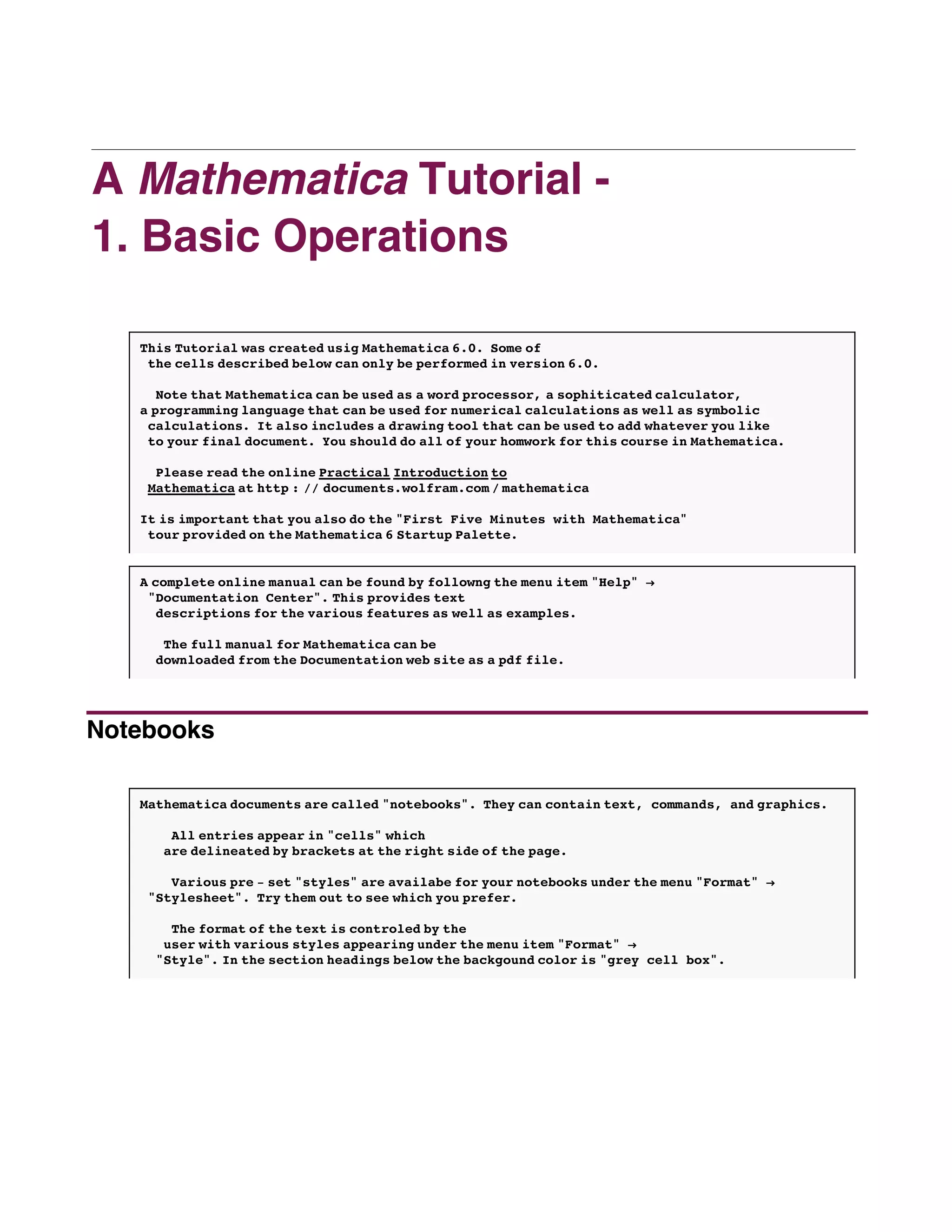
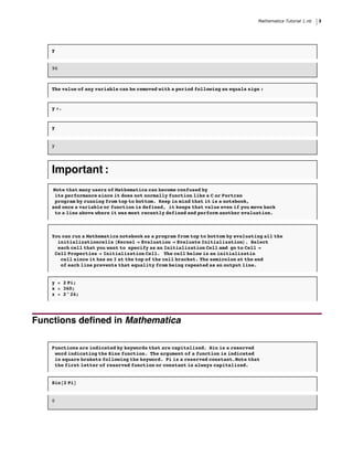
1) Mathematica notebooks contain cells for text, commands, and graphics. Functions are defined using capitalized keywords and arguments in brackets.
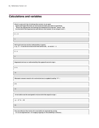
2) Basic calculations can be performed using standard operators like addition and multiplication. Variables can be assigned values.
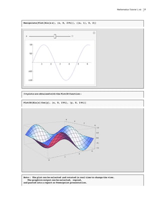
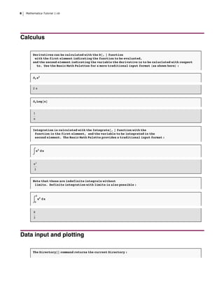
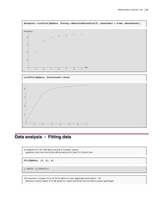
3) Plots of functions can be generated and manipulated using sliders. Calculus operations like derivatives and integrals are supported.
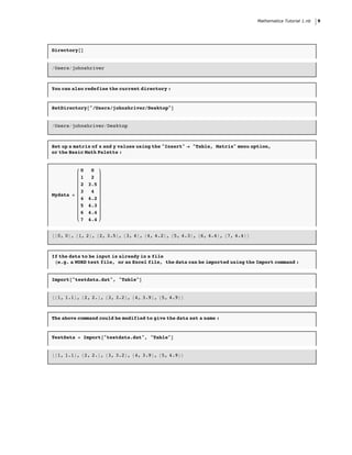
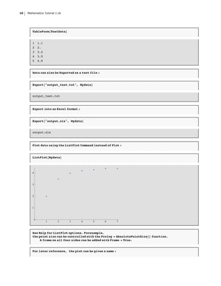
4) Data can be imported from files and exported for use in other programs. Basic plotting and analysis of data is demonstrated.
Mathematical Induction
CMSC 56 | Discrete Mathematical Structure for Computer Science
October 18, 2018
Instructor: Allyn Joy D. Calcaben
College of Arts & Sciences
University of the Philippines Visayas
In mathematics, graph theory is the study of graphs, which are mathematical structures used to model pairwise relations between objects.Graph theory is also important in real life.
Integration of GeoGebra in Teaching MathematicsNiroj Dahal
This presentation slide was prepared and presented by Niroj Dahal at Seventh National Conference on Mathematics and Its Applications at Butwal, Rupandehi, Nepal on January 12-15, 2019.
It contains the basics of matrix which includes matrix definition,types of matrices,operations on matrices,transpose of matrix,symmetric and skew symmetric matrix,invertible matrix,
application of matrix.
Introduction to Venn Diagrams and Sets. Includes the Operations: Intersection, Union, Complement.
If you would like a download of this PowerPoint then go to the following page:
http://passyworldofmathematics.com/pwerpoints/
A method for solving quadratic programming problems having linearly factoriz...IJMER
A new method namely, objective separable method based on simplex method is proposed for
finding an optimal solution to a quadratic programming problem in which the objective function can be
factorized into two linear functions. The solution procedure of the proposed method is illustrated with the
numerical example.
Sie halten das erste Jahrbuch des Historischen Museums Basel in den Händen. Jahrbuch deshalb, weil wir den bisherigen Jahresbericht inhaltlich ausgebaut und angereichert haben: Statt nur die Ereignisse des Vorjahres mit Enddatum am Jahresende retrospektiv aufzulisten, wagen wir auch einen Ausblick und erklären unseren eingeschlagenen Weg mit der zukunftsgerichteten eCulture-Strategie und lassen darin auch Mitarbeiterinnen und Mitarbeiter zu Wort kommen.
Der chronologisch erzählerische Rückblick in zwölf Monaten gewährt einen Blick hinter die Kulissen des Museumsalltags. Bewusst werden darin auch interne Aktivitäten erwähnt, um die Komplexität eines heutigen Museumsbetriebs zu dokumentieren. Arbeiten im Hintergrund, die sonst kaum wahrgenommen werden, oder auch aussergewöhnliche Schenkungen, von denen die Öffentlichkeit für gewöhnlich nicht hört, runden den Rückblick ab. Durch das HMB-Jahrbuch zieht sich erstmals eine Bildstrecke mit national und international bewegenden Momenten des letzten Jahres, die direkt oder indirekt Auswirkungen auf das Leben der Baslerinnen und Basler hatten und in Zukunft haben werden. Diese Bildstrecke illustriert die Verankerung des Museums in der Jetztzeit ebenso wie seine Rolle als urbanes Laboratorium, in dem ein interkulturelles Verständnis von Geschichte und Kulturerbe der Stadt ausgehandelt wird.
Selbstverständlich haben die traditionellen Kapitel zu Ausstellungen, Vermittlung, Publikationen, Zahlen und Fakten sowie dem als Lexikon konzipierten Sammlungszuwachs wie gewohnt ihren Platz. Wie üblich schliesst auch der Band 2014 mit dem Jahresbericht des Vereins für das Historische Museum Basel, der die Finanzierung dieser Publikation grosszügig unterstützt. Dafür danken wir dem Verein sehr!
Wir danken auch all unseren Gönnern, Donatoren, Sponsoren und Kooperationspartnern, ohne die unsere Arbeit schlicht nicht möglich wäre.
More instructions for the lab write-up1) You are not obli.docxgilpinleeanna
More instructions for the lab write-up:
1) You are not obligated to use the 'diary' function. It was presented only for you convenience. You
should be copying and pasting your code, plots, and results into some sort of "Word" type editor that
will allow you to import graphs and such. Make sure you always include the commands to generate
what is been asked and include the outputs (from command window and plots), unless the problem
says to suppress it.
2) Edit this document: there should be no code or MATLAB commands that do not pertain to the
exercises you are presenting in your final submission. For each exercise, only the relevant code that
performs the task should be included. Do not include error messages. So once you have determined
either the command line instructions or the appropriate script file that will perform the task you are
given for the exercise, you should only include that and the associated output. Copy/paste these into
your final submission document followed by the output (including plots) that these MATLAB
instructions generate.
3) All code, output and plots for an exercise are to be grouped together. Do not put them in appendix, at
the end of the writeup, etc. In particular, put any mfiles you write BEFORE you first call them.
Each exercise, as well as the part of the exercises, is to be clearly demarked. Do not blend them all
together into some sort of composition style paper, complimentary to this: do NOT double space.
You can have spacing that makes your lab report look nice, but do not double space sections of text
as you would in a literature paper.
4) You can suppress much of the MATLAB output. If you need to create a vector, "x = 0:0.1:10" for
example, for use, there is no need to include this as output in your writeup. Just make sure you
include whatever result you are asked to show. Plots also do not have to be a full, or even half page.
They just have to be large enough that the relevant structure can be seen.
5) Before you put down any code, plots, etc. answer whatever questions that the exercise asks first.
You will follow this with the results of your work that support your answer.
SAMPLE QUESTION:
Exercise 1: Consider the function
f (x,C)=
sin(C x)
Cx
(a) Create a vector x with 100 elements from -3*pi to 3*pi. Write f as an inline or anonymous function
and generate the vectors y1 = f(x,C1), y2 = f(x,C2) and y3 = f(x,C3), where C1 = 1, C2 = 2 and
C3 = 3. Make sure you suppress the output of x and y's vectors. Plot the function f (for the three
C's above), name the axis, give a title to the plot and include a legend to identify the plots. Add a
grid to the plot.
(b) Without using inline or anonymous functions write a function+function structure m-file that does
the same job as in part (a)
SAMPLE LAB WRITEUP:
MAT 275 MATLAB LAB 1 NAME: ...
Notebooks such as Jupyter give programming languages a level of interactivity approaching that of spreadsheets.
I present here an idea for a programming language specifically designed for an interactive environment similar to a notebook.
It aims to combining the power of a programming language with the usability of a spreadsheet.
Instead of free-form code, the user creates fields / columns, but these can be combined into tables and object classes.
By decoratively cycling through field elements, loops and other programming constructs can be created.
I give examples from classical computer science, machine learning and mathematical finance, specifically:
Nth Prime Number, 8 Queens, Poker Hand, Travelling Salesman, Linear Regression, VaR Attribution
1. Introduction to MATLAB and programming
2. Workspace, variables and arrays
3. Using operators, expressions and statements
4. Repeating and decision-making
5. Different methods for input and output
6. Common functions
7. Logical vectors
8. Matrices and string arrays
9. Introduction to graphics
10. Loops
11. Custom functions and M-files
I am Samuel H. I am a Mechanical Engineering Assignment Expert at matlabassignmentexperts.com. I hold a Ph.D. Matlab, University of Alberta, Canada. I have been helping students with their homework for the past 12 years. I solve assignments related to Mechanical Engineering.
Visit matlabassignmentexperts.com or email info@matlabassignmentexperts.com.
You can also call on +1 678 648 4277 for any assistance with Mechanical Engineering Assignments.
SAMPLE QUESTIONExercise 1 Consider the functionf (x,C).docxagnesdcarey33086
SAMPLE QUESTION:
Exercise 1: Consider the function
f (x,C)=
sin(C x)
Cx
(a) Create a vector x with 100 elements from -3*pi to 3*pi. Write f as an inline or anonymous function
and generate the vectors y1 = f(x,C1), y2 = f(x,C2) and y3 = f(x,C3), where C1 = 1, C2 = 2 and
C3 = 3. Make sure you suppress the output of x and y's vectors. Plot the function f (for the three
C's above), name the axis, give a title to the plot and include a legend to identify the plots. Add a
grid to the plot.
(b) Without using inline or anonymous functions write a function+function structure m-file that does
the same job as in part (a)
SAMPLE LAB WRITEUP:
MAT 275 MATLAB LAB 1 NAME: __________________________
LAB DAY and TIME:______________
Instructor: _______________________
Exercise 1
(a)
x = linspace(-3*pi,3*pi); % generating x vector - default value for number
% of pts linspace is 100
f= @(x,C) sin(C*x)./(C*x) % C will be just a constant, no need for ".*"
C1 = 1, C2 = 2, C3 = 3 % Using commans to separate commands
y1 = f(x,C1); y2 = f(x,C2); y3 = f(x,C3); % supressing the y's
plot(x,y1,'b.-', x,y2,'ro-', x,y3,'ks-') % using different markers for
% black and white plots
xlabel('x'), ylabel('y') % labeling the axis
title('f(x,C) = sin(Cx)/(Cx)') % adding a title
legend('C = 1','C = 2','C = 3') % adding a legend
grid on
Command window output:
f =
@(x,C)sin(C*x)./(C*x)
C1 =
1
C2 =
2
C3 =
3
(b)
M-file of structure function+function
function ex1
x = linspace(-3*pi,3*pi); % generating x vector - default value for number
% of pts linspace is 100
C1 = 1, C2 = 2, C3 = 3 % Using commans to separate commands
y1 = f(x,C1); y2 = f(x,C2); y3 = f(x,C3); % function f is defined below
plot(x,y1,'b.-', x,y2,'ro-', x,y3,'ks-') % using different markers for
% black and white plots
xlabel('x'), ylabel('y') % labeling the axis
title('f(x,C) = sin(Cx)/(Cx)') % adding a title
legend('C = 1','C = 2','C = 3') % adding a legend
grid on
end
function y = f(x,C)
y = sin(C*x)./(C*x);
end
Command window output:
C1 =
1
C2 =
2
C3 =
3
Joe Bob
Mon lab: 4:30-6:50
Lab 3
Exercise 1
(a) Create function M-file for banded LU factorization
function [L,U] = luband(A,p)
% LUBAND Banded LU factorization
% Adaptation to LUFACT
% Input:
% A diagonally dominant square matrix
% Output:
% L,U unit lower triangular and upper triangular such that LU=A
n = length(A);
L = eye(n); % ones on diagonal
% Gaussian Elimination
for j = 1:n-1
a = min(j+p.
Company Valuation webinar series - Tuesday, 4 June 2024FelixPerez547899
This session provided an update as to the latest valuation data in the UK and then delved into a discussion on the upcoming election and the impacts on valuation. We finished, as always with a Q&A
Digital Transformation and IT Strategy Toolkit and TemplatesAurelien Domont, MBA
This Digital Transformation and IT Strategy Toolkit was created by ex-McKinsey, Deloitte and BCG Management Consultants, after more than 5,000 hours of work. It is considered the world's best & most comprehensive Digital Transformation and IT Strategy Toolkit. It includes all the Frameworks, Best Practices & Templates required to successfully undertake the Digital Transformation of your organization and define a robust IT Strategy.
Editable Toolkit to help you reuse our content: 700 Powerpoint slides | 35 Excel sheets | 84 minutes of Video training
This PowerPoint presentation is only a small preview of our Toolkits. For more details, visit www.domontconsulting.com
Discover the innovative and creative projects that highlight my journey throu...dylandmeas
Discover the innovative and creative projects that highlight my journey through Full Sail University. Below, you’ll find a collection of my work showcasing my skills and expertise in digital marketing, event planning, and media production.
Personal Brand Statement:
As an Army veteran dedicated to lifelong learning, I bring a disciplined, strategic mindset to my pursuits. I am constantly expanding my knowledge to innovate and lead effectively. My journey is driven by a commitment to excellence, and to make a meaningful impact in the world.
Cracking the Workplace Discipline Code Main.pptxWorkforce Group
Cultivating and maintaining discipline within teams is a critical differentiator for successful organisations.
Forward-thinking leaders and business managers understand the impact that discipline has on organisational success. A disciplined workforce operates with clarity, focus, and a shared understanding of expectations, ultimately driving better results, optimising productivity, and facilitating seamless collaboration.
Although discipline is not a one-size-fits-all approach, it can help create a work environment that encourages personal growth and accountability rather than solely relying on punitive measures.
In this deck, you will learn the significance of workplace discipline for organisational success. You’ll also learn
• Four (4) workplace discipline methods you should consider
• The best and most practical approach to implementing workplace discipline.
• Three (3) key tips to maintain a disciplined workplace.
Business Valuation Principles for EntrepreneursBen Wann
This insightful presentation is designed to equip entrepreneurs with the essential knowledge and tools needed to accurately value their businesses. Understanding business valuation is crucial for making informed decisions, whether you're seeking investment, planning to sell, or simply want to gauge your company's worth.
Enterprise Excellence is Inclusive Excellence.pdfKaiNexus
Enterprise excellence and inclusive excellence are closely linked, and real-world challenges have shown that both are essential to the success of any organization. To achieve enterprise excellence, organizations must focus on improving their operations and processes while creating an inclusive environment that engages everyone. In this interactive session, the facilitator will highlight commonly established business practices and how they limit our ability to engage everyone every day. More importantly, though, participants will likely gain increased awareness of what we can do differently to maximize enterprise excellence through deliberate inclusion.
What is Enterprise Excellence?
Enterprise Excellence is a holistic approach that's aimed at achieving world-class performance across all aspects of the organization.
What might I learn?
A way to engage all in creating Inclusive Excellence. Lessons from the US military and their parallels to the story of Harry Potter. How belt systems and CI teams can destroy inclusive practices. How leadership language invites people to the party. There are three things leaders can do to engage everyone every day: maximizing psychological safety to create environments where folks learn, contribute, and challenge the status quo.
Who might benefit? Anyone and everyone leading folks from the shop floor to top floor.
Dr. William Harvey is a seasoned Operations Leader with extensive experience in chemical processing, manufacturing, and operations management. At Michelman, he currently oversees multiple sites, leading teams in strategic planning and coaching/practicing continuous improvement. William is set to start his eighth year of teaching at the University of Cincinnati where he teaches marketing, finance, and management. William holds various certifications in change management, quality, leadership, operational excellence, team building, and DiSC, among others.
Building Your Employer Brand with Social MediaLuanWise
Presented at The Global HR Summit, 6th June 2024
In this keynote, Luan Wise will provide invaluable insights to elevate your employer brand on social media platforms including LinkedIn, Facebook, Instagram, X (formerly Twitter) and TikTok. You'll learn how compelling content can authentically showcase your company culture, values, and employee experiences to support your talent acquisition and retention objectives. Additionally, you'll understand the power of employee advocacy to amplify reach and engagement – helping to position your organization as an employer of choice in today's competitive talent landscape.
1. A Mathematica Tutorial -
1. Basic Operations
This Tutorial was created usig Mathematica 6.0. Some of
the cells described below can only be performed in version 6.0.
Note that Mathematica can be used as a word processor, a sophiticated calculator,
a programming language that can be used for numerical calculations as well as symbolic
calculations. It also includes a drawing tool that can be used to add whatever you like
to your final document. You should do all of your homwork for this course in Mathematica.
Mathematica at http : êê documents.wolfram.com ê mathematica
Please read the online Practical Introduction to
It is important that you also do the "First Five Minutes with Mathematica"
tour provided on the Mathematica 6 Startup Palette.
A complete online manual can be found by followng the menu item "Help" Ø
"Documentation Center". This provides text
descriptions for the various features as well as examples.
The full manual for Mathematica can be
downloaded from the Documentation web site as a pdf file.
Notebooks
Mathematica documents are called "notebooks". They can contain text, commands, and graphics.
All entries appear in "cells" which
are delineated by brackets at the right side of the page.
Various pre - set "styles" are availabe for your notebooks under the menu "Format" Ø
"Stylesheet". Try them out to see which you prefer.
The format of the text is controled by the
user with various styles appearing under the menu item "Format" Ø
"Style". In the section headings below the backgound color is "grey cell box".
2. 2 Mathematica Tutorial 1.nb
Calculations and variables
Start a new cell by clicking the cursor in an open
space and type the text or calculation that you want to perform.
Start by typing the following followed by hitting the "enter" key
to evaluate the expression and obtain the answer in an output cell :
2 + 2
4
Multiplication can be indcated by a space,
e.g. 2 * 4 can be written with the asterisk, or with 2 ÿ 4
2ÿ4
8
Exponentiation is indicated by the upward carrot sign :
2^4
16
The most recent result of a calculation is symbolized by "%" :
2%
32
A variable can be assigned a value with the equals sign :
y = 2 ^ 6 + 32
96
it in an expression H or simply typing it followed by a returnL.
You can obtain the value of a variable at anytime by using
3. Mathematica Tutorial 1.nb 3
y
96
The value of any variable can be removed with a period following an equals sign :
y =.
y
y
Important :
Note that many users of Mathematica can become confused by
its performance since it does not normally function like a C or Fortran
program by running from top to bottom. Keep in mind that it is a notebook,
and once a variable or function is defined, it keeps that value even if you move back
to a line above where it was most recently defined and perform another evaluation.
initializationcells HKernel Ø Evaluation Ø Evaluate InitializationL. Select
You can run a Mathematica notebook as a program from top to bottom by evaluating all the
each cell that you want to specify as an Initialization Cell amd go to Cell Ø
Cell Properties Ø Initialization Cell. The cell below is an initializatin
cell since it has an I at the top of the cell bracket. The semicolon at the end
of each line prevents that equality from being repeated as an output line.
y = 2 Pi;
x = 360;
z = 2 ^ 24;
Functions defined in Mathematica
Functions are indicated by keywords that are capitalized. Sin is a reserved
word indicating the Sine function. The argument of a function is indicated
in square brakets following the keyword. Pi is a reserved constant.Note that
the first letter of reserved function or constant is always capitalized.
Sin@2 PiD
0
4. 4 Mathematica Tutorial 1.nb
The argument of trig functions is in radians by default.
Sin@Pi ê 2D
1
argument HNote the unit Degree is always singular in MathematicaL :
You can switch to degrees by writing "Degree" after the
Sin@90 DegreeD
1
Numerical evaluation can be forced with the N@D function :
Pi
p
N@PiD
3.14159
The level of precision can be specified as a second element in the N function.
N@Pi, 100D
3.1415926535897932384626433832795028841971693993751058209749445923078164062862089986280Ö
34825342117068
Functions defined by the user
You can define our own functions. Note that the definition specifies the
variable on the left side in brackets with the underline following it. This is to
be substituted into the expression on the right. The function can be used anywhere
it is needed with the value for the variable explicitly indicated in brackets.
ANewFunc@x_D := x ^ 2 + 2 x + 3
5. Mathematica Tutorial 1.nb 5
y = ANewFunc@20D
443
The definition of any function can be removed with an equals sign followed by a period :
ANewFunc@x_D =.
y = ANewFunc@20D
ANewFunc@20D
Logarithms
The natural log of a number is obtained with the Log@D function :
Log@10.0D
2.30259
The log of a number to the base 10 is obtained with the Log@10, xD :
Log@10, 2.0D
0.30103
Plotting
Use the Plot function to plot the a function,
with the limits for the plot indicated in curly brakets :
6. 6 Mathematica Tutorial 1.nb
Plot@Sin@xD, 8x, 0, 2 Pi<D
1
0.5
1 2 3 4 5 6
-0.5
-1
Ü Graphics Ü
See the online documentation and manual for more complete control of axes and labels.
Plot@Log@xD, 8x, 0, 6<D
2
1 2 3 4 5 6
-2
-4
-6
-8
Ü Graphics Ü
The Manipulate command permits the addition of a slide bar to a
plot to allow real time adjustment of parameters. In the example below,
the parameter is adjustable from 0 to 2 with the initial value set to 1.
7. Mathematica Tutorial 1.nb 7
Manipulate@Plot@Sin@n xD, 8x, 0, 2 Pi<D, 88n, 1<, 0, 2<D
n
1.0
0.5
1 2 3 4 5 6
-0.5
-1.0
3 D plots are obtained with the Plot3D function :
Plot3D@Sin@xD Cos@yD, 8x, 0, 2 Pi<, 8y, 0, 2 Pi<D
Note : The plot can be selected and rotated in real time to change the view.
The graphics output can be selected, copied,
and pasted into a report or Powerpoint presentation.
Calculus
8. 8 Mathematica Tutorial 1.nb
Calculus
Derivatives can be calculated with the D@, D function
with the first element indicating the function to be evaluated,
to. Use the Basic Math Palettes for a more traditional input format Has shown hereL :
and the second element indicating the variable the derivative is to be caluclated with respect
∂x x2
2x
∂x Log@xD
1
x
Integration is calculated with the Integrate@, D function with the
function in the first element, and the variable to be integrated in the
second element. The Basic Math Palette provides a traditional input format :
‡ x „x
2
x3
3
Note that these are indefinite integrals without
limits. Definite integration with limits is also possible :
‡ x „x
2
2
0
8
3
Data input and plotting
The Directory@D command returns the current Directory :
9. Mathematica Tutorial 1.nb 9
Directory@D
êUsersêjohnshriver
You can also redefine the current directory :
SetDirectory@"êUsersêjohnshriverêDesktop"D
êUsersêjohnshriverêDesktop
Set up a matrix of x and y values using the "Insert" Ø "Table, Matrix" menu option,
or the Basic Math Palette :
0 0
1 2
2 3.5
3 4
Mydata =
4 4.2
5 4.3
6 4.4
7 4.4
880, 0<, 81, 2<, 82, 3.5<, 83, 4<, 84, 4.2<, 85, 4.3<, 86, 4.4<, 87, 4.4<<
He.g. a WORD text file, or an Excel file, the data can be imported using the Import command :
If the data to be input is already in a file
Import@"testdata.dat", "Table"D
881, 1.1<, 82, 2.<, 83, 3.2<, 84, 3.9<, 85, 4.9<<
The above command could be modified to give the data set a name :
TestData = Import@"testdata.dat", "Table"D
881, 1.1<, 82, 2.<, 83, 3.2<, 84, 3.9<, 85, 4.9<<
10. 10 Mathematica Tutorial 1.nb
TableForm@TestDataD
1 1.1
2 2.
3 3.2
4 3.9
5 4.9
Data can also be Exported as a text file :
Export@"output_test.txt", MydataD
output_test.txt
Export into an Excel format :
Export@"output.xls", MydataD
output.xls
Plot data using the ListPlot Command instead of Plot :
ListPlot@MydataD
4
3
2
1
1 2 3 4 5 6 7
See Help for ListPlot options. Forexample,
the point size can be controlled with the Prolog Ø AbsolutePointSize@D function.
A frame on all four sides can be added with Frame Ø True.
For later reference, the plot can be given a name :
11. Mathematica Tutorial 1.nb 11
dataplot = ListPlot@Mydata, Prolog Ø AbsolutePointSize@5D, AxesLabel Ø 8time, absorbance<D
absorbance
4
3
2
1
time
1 2 3 4 5 6 7
ListPlot@Mydata, PlotJoined Ø TrueD
4
3
2
1
1 2 3 4 5 6 7
Data analysis - Fitting data
A simple fit of the data using a linear least
square routine could be obtained with the Fit function.
Fit@Mydata, 81, x<, xD
1.45833 + 0.540476 x
Of course a linear fit of this data is not appropriate here. To
obtain a nonlinear fit we need to load the Statistics Nonlinear package.
12. 12 Mathematica Tutorial 1.nb
Needs@"NonlinearRegression`"D;
NonlinearFit@data, model, 8parameters<, 8variables<D
The function NonlinearFit requires the following format :
The model is the mathematical function which is assumed to describe
the data. The list of variables and parameters follow. Typically,
the variables list will only contain a single variable,
while the parameters to be fit may contain two or more items.
Hof course a linear fit would normally be accomplished the linear least squares program Fit@D,
A simple example would be a fit of the above data with a linear equation
but it works here as an introductory exampleL.
NonlinearRegress@Mydata, a + b x, 8a, b<, xD
:BestFitParameters Ø 8a Ø 1.45833, b Ø 0.540476<,
80.00911456, 2.90755< ,
Estimate Asymptotic SE CI
80.194047, 0.886906<
ParameterCITable Ø a 1.45833 0.592264
b 0.540476 0.141578
EstimatedVariance Ø 0.841865,
DF SumOfSq MeanSq
Model 2 102.049 51.0244
ANOVATable Ø Error 6 5.05119 0.841865 ,
Uncorrected Total 8 107.1
Corrected Total 7 17.32
1. -0.83666
AsymptoticCorrelationMatrix Ø ,
-0.83666 1.
Curvature
>
Max Intrinsic 0
FitCurvatureTable Ø
Max Parameter-Effects 0
95. % Confidence Region 0.440942
Hthe user usually knows what function to fit the data to based on the experimental situation,
A more appropriate function is normally obtained from an understanding of the experiment
alternatively, he can fit the data to an arbitrary function, e.g. a polynomialL.
13. Mathematica Tutorial 1.nb 13
NonlinearRegress@Mydata, a x ê Hx + bL, 8a, b<, xD
:BestFitParameters Ø 8a Ø 5.4583, b Ø 1.33173<,
84.7451, 6.1715<
Estimate Asymptotic SE CI
80.692517, 1.97095<
ParameterCITable Ø a 5.4583 0.291469 ,
b 1.33173 0.261235
EstimatedVariance Ø 0.0440968,
DF SumOfSq MeanSq
Model 2 106.835 53.4177
ANOVATable Ø Error 6 0.264581 0.0440968 ,
Uncorrected Total 8 107.1
Corrected Total 7 17.32
1. 0.924797
AsymptoticCorrelationMatrix Ø ,
0.924797 1.
Curvature
>
Max Intrinsic 0.0735356
FitCurvatureTable Ø
Max Parameter-Effects 0.248355
95. % Confidence Region 0.440942
A plot of the fitted function Hwith the plot given a name "fit" hereL :
fit = Plot@5.45833 x ê H1.33177 + xL, 8x, 0, 7<D
4
3
2
1
1 2 3 4 5 6 7
Overlay the data and the fitted function with the Show function :