Here is a MATLAB script to solve the quadratic equation with variable coefficients: % Script to solve the quadratic equation ax^2 + bx + c = 0 clear disp('Enter coefficients a, b, c: ') a = input('a = '); b = input('b = '); c = input('c = '); x = sym('x'); sol = solve(a*x^2 + b*x + c == 0, x); disp('The solutions are:') disp(sol) This script first clears any existing variables, then prompts the user to input the coefficients a, b, and c. It then defines x as a symbolic variable

1. Introduction to MATLAB
1
Lecture-1

2. 2
Objectives
 Background of MATLAB
 Advantages and disadvantages
 Applications
 Basic commands, syntax
 Introduction to decimal places, rounding, significant figures
 Solve problems using different mathematical methods

3. 3
Background of MATLAB
 It stands for matrix laboratory
 It is a technical programming language
 Superior to other language such as C, FORTRAN
 A special purpose of computer program optimized to perform
engineering and scientific calculations
 It provides very extensive library of predefined functions to
make technical programming task easier and efficient.

4. 4
Advantages and Disadvantages of MATLAB
Advantages:
 Easy to use
 Independent platform
 Pre-defined functions
 Device independent plotting
 Graphical user interface
Disadvantages:
 Computing speed is slow
 Cost effective for business

5. 5
Applications
 Technical computing
 Control design
 Communications design
 Test and Measurement
 Image processing
 Signal processing
 Chemical Industry
 Financial modelling and Analysis

6. 6
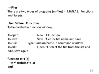
Basic commands and Syntax
Simple computation may be carried out in the Command Window
by entering an instruction at the prompt. Commands and names are
case sensitive.
# Used fixed constant (Example-pi())
# Built-in Functions
Mathematical functions are available with commonly used name.
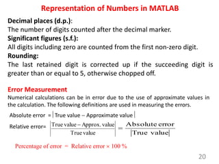
Note the following change:
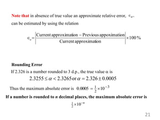
log() natural logarithm(ln), log10() log base 10
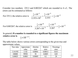
Percent (%) sign is used to write comments.
Semicolon (;) at the end of command suppress the output.
# Matrices
All variables in MATLAB are treated as matrices or arrays.
A row vector may be entered as
>> x=[1 2 3] or x=[1,2,3]
Output x =
1 2 3

7. 7
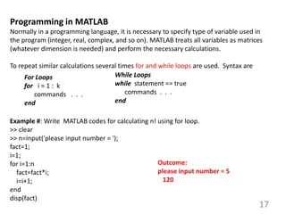
A column vector may be entered as
>> y = [4; 5; 6] or y = [4 5 6]’
Output y =
4
5
6
# Semicolons are used to separate the rows of a matrix.
An example of a 3-by-4 matrix is B = [1 2 3 4; 5 6 7 8; 9 10 11 12]
# Using colon (:)
Example- x=1:5 %Generates a vector with interval of 1 from
1 to ≤ 5
# Use linspace
Example-linspace (a, b, n) % generate n values in [a, b] with
equal length
x2 = linspace(1,2.5,4)
Output x2 =
1 1.5 2 2.5

8. 8
Controlling number of digits
The fixed-point numbers:
format short displays 5 digits
format long displays 16 digits
The floating-point representation:
format short e gives 5 digits plus the exponent
format long e gives 16 digits plus the exponent
The combined format (fixed point or floating depending on the
magnitude of the number)
format short g
format long g

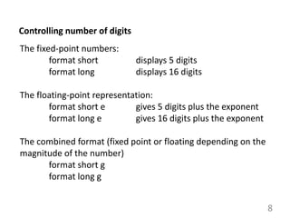
9. 9
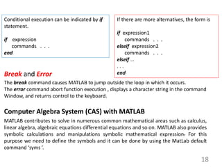
Printing command in MATLAB
1. By typing the name of a variable (displays the output indicating
variable name).
Example- write the new script then save as “.m” file.
clear
>>A=[1, 2.25 4.56];
>> A
A =
1.0000 2.2500 4.5600
2. By using “disp” built in function. This displays output without
variable name.
>>disp(A)
1.0000 2.2500 4.5600
3. By using “fprintf “ function
Syntax: fprintf(formatSpec, A1, A2, . . . , A3)

10. 10
Printing command in MATLAB
Example-
>>clear
>> x=0:0.5:2;
>> y=sin(x);
>>fprintf('%6s %12sn','x','sin(x)');
x sin(x)
0.00 0.000000
0.50 0.479426
1.00 0.841471
1.50 0.997495
2.00 0.909297

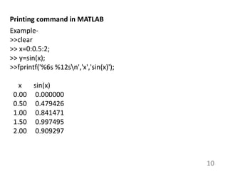
11. 11
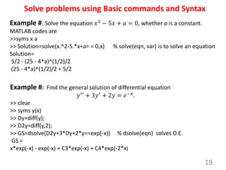
Plotting command in MATLAB
7cos 2 1
y x x
  
2-D Plot
plot(y) x = 1 : n (if not supplied)
plot(x,y) x, y are vectors
plot(x1, y1, . . .. , xn,Yn)
title(‘plot title’) grid on grid off
xlabel(‘label for x-axis’) grid (toggles)
ylabel(‘label for y-axis’) hold on hold off
box on
Example #. Plot the function in [-4,4].
>> x= -4:0.2:4;
>> y=7*cos(x)+2*x-1;
>> plot(x,y);grid on

12. 12
Plotting command in MATLAB
3-D Plot
plot3(x,y,z) % Command
Example #. Plot the function
>> x=linspace(-5,5,50);
>> y=x;
>> z=4-x.^2-y.^2;
>> plot3(x,y,z); grid on;
2 2
4
z x y
  
Construction of Functions in the Command Window
1. Inline function
f1 =jnline(expr)
f2=inline(expr, arg1, arg2,. . . )
Example
>> f=inline('x^2+2*x*y')
f =
Inline function:
f(x,y) = x^2+2*x*y
>> v1=f(1, 2.2)
Result
v1 =
5.4000

13. 13
Construction of Functions in the Command Window
2. Function_handle (@) )
handle=@(arglist) anonymous_function
Example
>> ff=@(x,y) x.^2+x./y
ff =
@(x,y)x.^2+x./y
>> ff(1.1,2)
ans =
1.7600
3. Function using Symbols
>> syms x y
>> ff(x,y)=x.^2+x./y
ff(x, y) =
x^2 + x/y
To compute elementwise in array use
POWER with (.^) , DIVISION with (./) and PTRODUCT with (.*)
>> ff(1.2, 2) % returns result in fracttion
ans =
51/25
>> ffval=eval(ff(1.2,2)) % eval( ) is used to convert fraction
to decimal form
ffval =
2.04

14. 14
m-Files
There are two types of programs (m-files) in MATLAB: Functions
and Scripts.
User Defined Functions
To be created in function window.
To open: New  Function
To save: Save  enter file name and save
To run: Type function name in command window
To edit: Open  select the file from the list and
edit. save again
function t=FF(a)
t=7*cos(a)+2*a-1;
end

15. 15
m-Files
The function which is created as an m-file and saved as FF.m.
To use the above function type in command window.
>> t=FF(2)
t =
0.0870
Scripts
Scripts provide a set of MATLAB commands, comments, values,
plotting commands, and so on.
A scripts that has been created and saved is executed by typing the file
name at the MATLAB prompt in the command window or using save and
run from the Debug menu.
To open: New  Script
To save: Save  enter file name and save
To run: Type script name in command window
To edit: Open  select the file from the list and edit. Save again

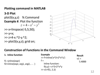
16. 16
Scripts
% Script TestProgm
%Values of f(x) for different values of x
x= x0;
disp('n xn f(xn)')
for i=1:nmax
fx=f(x);
n=i-1;
disp([n,x,fx])
x=x+h;
end
Save the script as TestProg.m
To execute the script from Command Window,
type following commands:
>> clear
>> x0=1;
>> h=0.5;
>> f=inline('7.*cos(x)+2.*x-1')
f =
Inline function:
f(x) = 7*cos(x)+2*x-1
>> nmax=5
nmax =
5
>> TestProg % Type the Script name
Output
n xn f(xn)
0 1.0000 4.7821
1.0000 1.5000 2.4952
2.0000 2.0000 0.0870
3.0000 2.5000 -1.6080
4.0000 3.0000 -1.9299

17. 17
Programming in MATLAB
Normally in a programming language, it is necessary to specify type of variable used in
the program (integer, real, complex, and so on). MATLAB treats all variables as matrices
(whatever dimension is needed) and perform the necessary calculations.
To repeat similar calculations several times for and while loops are used. Syntax are
While Loops
while statement == true
commands . . .
end
For Loops
for i = 1 : k
commands . . .
end
Example #: Write MATLAB codes for calculating n! using for loop.
>> clear
>> n=input('please input number = ');
fact=1;
i=1;
for i=1:n
fact=fact*i;
i=i+1;
end
disp(fact)
Outcome:
please input number = 5
120

18. 18
Conditional execution can be indicated by if
statement.
if expression
commands . . .
end
The break command causes MATLAB to jump outside the loop in which it occurs.
The error command abort function execution , displays a character string in the command
Window, and returns control to the keyboard.
If there are more alternatives, the form is
if expression1
commands . . .
elseif expression2
commands . . .
elseif …
. . .
end
Break and Error
MATLAB contributes to solve in numerous common mathematical areas such as calculus,
linear algebra, algebraic equations differential equations and so on. MATLAB also provides
symbolic calculations and manipulations symbolic mathematical expression. For this
purpose we need to define the symbols and it can be done by using the MatLab default
command ‘syms ’.
Computer Algebra System (CAS) with MATLAB

19. 19
Solve problems using Basic commands and Syntax
Example #: Solve the equation 𝑥2 − 5𝑥 + 𝑎 = 0, whether a is a constant.
MATLAB codes are
>>syms x a
>> Solution=solve(x.^2-5.*x+a= = 0,x) % solve(eqn, var) is to solve an equation
Solution=
5/2 - (25 - 4*a)^(1/2)/2
(25 - 4*a)^(1/2)/2 + 5/2
Example #: Find the general solution of differential equation
𝑦′′
+ 3𝑦′
+ 2𝑦 = 𝑒−𝑥
.
>> clear
>> syms y(x)
>> Dy=diff(y);
>> D2y=diff(y,2);
>> GS=dsolve(D2y+3*Dy+2*y==exp(-x)) % dsolve(eqn) solves D.E.
GS =
x*exp(-x) - exp(-x) + C3*exp(-x) + C4*exp(-2*x)

20. 20
Representation of Numbers in MATLAB
Percentage of error = Relative error  100 %
Decimal places (d.p.):
The number of digits counted after the decimal marker.
Significant figures (s.f.):
All digits including zero are counted from the first non-zero digit.
Rounding:
The last retained digit is corrected up if the succeeding digit is
greater than or equal to 5, otherwise chopped off.
Error Measurement
Numerical calculations can be in error due to the use of approximate values in
the calculation. The following definitions are used in measuring the errors.
Absolute error =True value  Approximate value
value
True
value
Approx.
value
True 
value
True
error
Absolute

Relative error=

21. 21
%
100
ion
approximat
Current
on
appoximati
Previous
ion
approximat
Current



a
can be estimated by using the relation
,
a

Note that in absence of true value an approximate relative error,
3
2
1 10
0005
.
0 


Rounding Error
If 2.326 is a number rounded to 3 d.p., the true value  is
2.3255 2.3265or 2.326 0.0005
 
   
n

10
2
1
Thus the maximum absolute error is
If a number is rounded to n decimal places, the maximum absolute error is

22. 22
Consider two numbers 235.3 and 0.003267 which are rounded to 4 s.f.. The
errors can be estimated as follows
For 235.3, the relative error is 3
2
1
3
2
1
2
1
2
1
10
353
.
2
10
10
353
.
2
10 








For 0.003267. the relative error is 3
2
1
3
2
1
3
6
2
1
10
267
.
3
10
10
267
.
3
10 









In general, if a number is rounded to n significant figures the maximum
relative error is 1
1
2 10 .
n
 

The table below shows various errors corresponding to the given true and
approximate values.
True value Approximate
value
Absolute
error
Relative
error
Percentage
error
3.141592 3.142 0.00041 0.00013 0.013
100000 99950 50 0.0005 0.05
0.00025 0.0003 0.00005 0.2 20

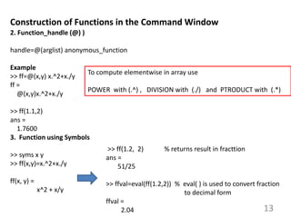
23. 23
Solve problems using Basic commands and Syntax
Example #: 0
2


 c
bx
ax
The solution of the quadratic equation
is )
2
(
)
4
( /
2
a
ac
b
b
x 



Write a MATLAB script to solve the quadratic equation with variable coefficients
which gives variable significant digits.
Solution:
% Script QuadEq for solution
clear all
disp('Solution of Quadratic Equation')
% Equation : ax^2+bx+c=0
% Roots: x1= -b+sqrt(b^2-4ac)/(2a)
% x2= -b-sqrt(b^2-4ac)/(2a)
abc=input('Supply a,b,c as [a,b,c]=');
a=abc(1); b=abc(2); c=abc(3);
x1=(-b+sqrt(b^2-4*a*c))/(2*a);
x2=(-b-sqrt(b^2-4*a*c))/(2*a);
Roots=[x1,x2]
disp('Roots to n significant digits')
n=input('Value of n = ');
Roots_n=vpa([x1; x2],n)

24. 24
Try to do yourself
Outcomes
 Numerically solve problems by using different mathematical
methods, built in function in MATLAB
 Visualization problems by data analysis
 Save time for solve problems
Exercise 1:Write script and solve the following equation then correct
it to ten significant figures.
2
6 9886 1 0
x x
  
𝑦′′
− 2𝑦′
+ 10𝑦 = 5𝑥 − 𝑒3𝑥
Exercise 2:Find the general solution of the following ordinary
differential equation (ODE)

25. 25
Calculate the Celsius temperature by using the following relation
between 𝐹 and 𝐶
Exercise 3:
𝐹 − 32
180
=
𝐶
100
where the range of Fahrenheit temperatures from 10 to 200 with interval 5.
Then print these values with the proper headings by using the “fprintf” command
in MATLAB.
References
Text Book:
Applied Numerical Methods with MATLAB for Engineers and Scientists- S.C. Chapra,
4th Edition, 2017, McGraw Hill-Europe.
Reference Book:
Numerical Methods in Engineering with MATLAB – Jaan Kiusalaas, 4th Edition, 2018,
CAMBRIDGE UNIVERSITY PRESS, UK.
Applied Numerical Methods With Matlab for Engineers and Scientists ( Steven
C.Chapra).