POLYTECHNIC UNGKU OMAR
                           ELECTRICAL ENGINEERING DEPARTMENT
Course         :      E5124 DATA COMMUNICATION (Lab work)
Experiment     :      Matlab 1 – Get Familiarize (Matrices and Plot)


The objective of this session is to learn:
       - How to launch the matlab software
       - Few simple calculations and formulation
       - Plot command and graphical output


Introduction

Matlab is a tool for doing numerical computations with matrices and vectors. It can also display information
graphically. The best way to learn what Matlab can do is to work through some examples at the computer. After
reading and familiarize with this exercise you will be able to solve construct own work.


Starting MATLAB


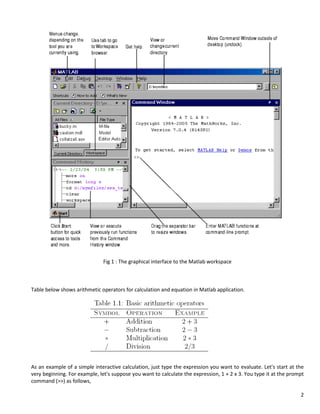
Launch MATLAB by double-clicking on the MATLAB icon on your Windows desktop. When you start MATLAB, a
special window called the MATLAB desktop appears. The desktop is a window that contains other windows. The
major tools within or accessible from the desktop are (refer Fig 1):
        - The Command Window
        - The Command History
        - The Workspace
        - The Current Directory
        - The Help Browser
        - The Start button


                                                                                                             1
Fig 1 : The graphical interface to the Matlab workspace


Table below shows arithmetic operators for calculation and equation in Matlab application.


As an example of a simple interactive calculation, just type the expression you want to evaluate. Let's start at the
very beginning. For example, let's suppose you want to calculate the expression, 1 + 2 x 3. You type it at the prompt
command (>>) as follows,

                                                                                                                   2
>> 1+2*3

                 ans =
                          7

You will have noticed that if you do not specify an output variable, MATLAB uses a default variable ans, short for
answer, to store the results of the current calculation. Note that the variable ans is created (or overwritten, if it is
already existed). To avoid this, you may assign a value to a variable or output argument name. For example,
                >> x = 1+2*3

                 x=
                          7

will result in x being given the value 1 + 2 x 3 = 7. This variable name can always be used to refer to the results of the
previous computations. Therefore, computing 4x will result in
                  >> 4*x

                 ans =
                          28.0000


Exercise
1.      Matrix

1.1     Insert the following expression and observe the result.

        >>aa=[l 3 4; 5 7 8; 2 3 5]
        Observation


        >> y=[10; 9; 8]
        Observation


                                                                                                                        3
1.2   Insert both expressions.

              >>aa=[l 3 4; 5 7 8; 2 3 5];
              >> y=[10; 9; 8];

      Now obtain result for following expression
             >>aay
      Observation


             >>inv(aa)*y
      Observation


             >> [inv(aa)*y aay]
      Observation


      Explain your observation for expression [inv(aa)*y aay]

      _____________________________________________________________________________________

      _____________________________________________________________________________________


2.    Matrix Loop

2.1   Insert following expression and obtain result


                                                                                              4
>> a = [ 0.8 0.1; 0.2 0.9 ]
      Observation


      >> x = [ 1; 0 ]
      Observation


2.2   Type below expression and state your observation
      >> a = [ 0.8 0.1; 0.2 0.9 ];
      >> x = [ 1; 0 ];
      >> for i = 1:20, x = a*x, end

      Observation


                                                         5
3.    Plot

      MATLAB has an excellent set of graphic tools. Plotting a given data set or the results of computation is
      possible with very few commands. You are highly encouraged to plot mathematical functions and results of
      analysis as often as possible. Trying to understand mathematical equations with graphics is an enjoyable and
      very e±cient way of learning mathematics. Being able to plot mathematical functions and data freely is the
      most important step, and this section is written to assist you to do just that.

3.1   Let say, your given few samples of variable which need to find out their performance rate. Now, insert following
      expression:-
              >> a=[1 2 3 4 6 4 3 4 5]

      Observation


             >> b=a+2
      Observation


3.2   Use plot command to plot your result.

             >> plot(b)
      Observation


             >> grid on
      Observation


                                                                                                                    6
3.3   Use label and title command to provide information at graph. Type this command step by step in order to
      observe result. Before you type command, display your Matlab window panel and graph window side by
      side in order to get better view.

              >> xlabel('Sequence of b')
              >> ylabel('b value')
              >> title(‘Graphical output for b sequence of number’)

      Observation


3.4   Bar command used to plot bar graph which able to show us the statistical result.

              >> bar(b)
              >> xlabel('Number of sample')
              >> ylabel('Weight of random samples in kg')

      Observation


                                                                                                           7
>> plot(b,'*')
>> axis([0 12 0 10])

        Observation


        What did you see from both graphs? Explain.

        ______________________________________________________________________________________

        ______________________________________________________________________________________


3.5     To make a graph of y = sin(t) on the interval t = 0 to t = 10, do the following steps:
                       >> t = 0:.3:10;
                       >> y = sin(t);
                       >> plot(t,y)
                       >> title('Sine wave ')
                       >> xlabel(‘Time, t')
                       >> ylabel('Amplitude')

        Observation


                                                                                                 8
3.6      Plotting multiple wave or result in single graph. Execute following command and make your observation.
         Insert title and label by yourself.

>> t=0:0.1:30;
>> y1=sin(t);
>> y2=cos(t);
>> plot(t,y1,'--',t,y2,'-r')
        Observation


>> t=0:0.1:30;
>> y1=sin(t).*t;
>> y2=cos(t).*t;
>> plot(t,y1,'--',t,y2,'-r')
        Observation


                                                                                                                  9
3.7   Subplot
      The subplot is used to put multiple plots on the same MATLAB figure window.
              subplot(pqr) - p & q represent matrixes, r locating position for plotted graph
      a) Write the following expression and obtain the result.

               >> x = 0 : 0.1 : 3 *pi;
               >> y = sin(x);
               >> z = cos(x);
               >> subplot(222)
               >> plot(x,y)
               >> title('Sine wave y')
               >> xlabel('time, x')
               >> ylabel('Amplitude, y')
               >> subplot(223)
               >> title('x and z')
               >> subplot(224)
               >> plot(x,y,'-',x,z,' -- ')
               >> title('x and [y z]')

      b) Once complete your subplot, insert label and title for each graph individually. Use example as given in
         above command.
         Observation


                                                                                                             10
c) Discrete sample graphical output.
          Type following command and make observation. State the differences between both results.

                >> p=0:0.05:5;
                >> q=sin(p.^2);
                >> plot(p,q);

       Observation


                >> p=0:0.05:5;
                >> q=sin(p.^2);
                >> stem(p,q);

       Observation


Reflection

_____________________________________________________________________________________________

_____________________________________________________________________________________________

_____________________________________________________________________________________________

_____________________________________________________________________________________________


                                                                                                     11

Matlab 1

  • 1.
    POLYTECHNIC UNGKU OMAR ELECTRICAL ENGINEERING DEPARTMENT Course : E5124 DATA COMMUNICATION (Lab work) Experiment : Matlab 1 – Get Familiarize (Matrices and Plot) The objective of this session is to learn: - How to launch the matlab software - Few simple calculations and formulation - Plot command and graphical output Introduction Matlab is a tool for doing numerical computations with matrices and vectors. It can also display information graphically. The best way to learn what Matlab can do is to work through some examples at the computer. After reading and familiarize with this exercise you will be able to solve construct own work. Starting MATLAB Launch MATLAB by double-clicking on the MATLAB icon on your Windows desktop. When you start MATLAB, a special window called the MATLAB desktop appears. The desktop is a window that contains other windows. The major tools within or accessible from the desktop are (refer Fig 1): - The Command Window - The Command History - The Workspace - The Current Directory - The Help Browser - The Start button 1
  • 2.
    Fig 1 :The graphical interface to the Matlab workspace Table below shows arithmetic operators for calculation and equation in Matlab application. As an example of a simple interactive calculation, just type the expression you want to evaluate. Let's start at the very beginning. For example, let's suppose you want to calculate the expression, 1 + 2 x 3. You type it at the prompt command (>>) as follows, 2
  • 3.
    >> 1+2*3 ans = 7 You will have noticed that if you do not specify an output variable, MATLAB uses a default variable ans, short for answer, to store the results of the current calculation. Note that the variable ans is created (or overwritten, if it is already existed). To avoid this, you may assign a value to a variable or output argument name. For example, >> x = 1+2*3 x= 7 will result in x being given the value 1 + 2 x 3 = 7. This variable name can always be used to refer to the results of the previous computations. Therefore, computing 4x will result in >> 4*x ans = 28.0000 Exercise 1. Matrix 1.1 Insert the following expression and observe the result. >>aa=[l 3 4; 5 7 8; 2 3 5] Observation >> y=[10; 9; 8] Observation 3
  • 4.
    1.2 Insert both expressions. >>aa=[l 3 4; 5 7 8; 2 3 5]; >> y=[10; 9; 8]; Now obtain result for following expression >>aay Observation >>inv(aa)*y Observation >> [inv(aa)*y aay] Observation Explain your observation for expression [inv(aa)*y aay] _____________________________________________________________________________________ _____________________________________________________________________________________ 2. Matrix Loop 2.1 Insert following expression and obtain result 4
  • 5.
    >> a =[ 0.8 0.1; 0.2 0.9 ] Observation >> x = [ 1; 0 ] Observation 2.2 Type below expression and state your observation >> a = [ 0.8 0.1; 0.2 0.9 ]; >> x = [ 1; 0 ]; >> for i = 1:20, x = a*x, end Observation 5
  • 6.
    3. Plot MATLAB has an excellent set of graphic tools. Plotting a given data set or the results of computation is possible with very few commands. You are highly encouraged to plot mathematical functions and results of analysis as often as possible. Trying to understand mathematical equations with graphics is an enjoyable and very e±cient way of learning mathematics. Being able to plot mathematical functions and data freely is the most important step, and this section is written to assist you to do just that. 3.1 Let say, your given few samples of variable which need to find out their performance rate. Now, insert following expression:- >> a=[1 2 3 4 6 4 3 4 5] Observation >> b=a+2 Observation 3.2 Use plot command to plot your result. >> plot(b) Observation >> grid on Observation 6
  • 7.
    3.3 Use label and title command to provide information at graph. Type this command step by step in order to observe result. Before you type command, display your Matlab window panel and graph window side by side in order to get better view. >> xlabel('Sequence of b') >> ylabel('b value') >> title(‘Graphical output for b sequence of number’) Observation 3.4 Bar command used to plot bar graph which able to show us the statistical result. >> bar(b) >> xlabel('Number of sample') >> ylabel('Weight of random samples in kg') Observation 7
  • 8.
    >> plot(b,'*') >> axis([012 0 10]) Observation What did you see from both graphs? Explain. ______________________________________________________________________________________ ______________________________________________________________________________________ 3.5 To make a graph of y = sin(t) on the interval t = 0 to t = 10, do the following steps: >> t = 0:.3:10; >> y = sin(t); >> plot(t,y) >> title('Sine wave ') >> xlabel(‘Time, t') >> ylabel('Amplitude') Observation 8
  • 9.
    3.6 Plotting multiple wave or result in single graph. Execute following command and make your observation. Insert title and label by yourself. >> t=0:0.1:30; >> y1=sin(t); >> y2=cos(t); >> plot(t,y1,'--',t,y2,'-r') Observation >> t=0:0.1:30; >> y1=sin(t).*t; >> y2=cos(t).*t; >> plot(t,y1,'--',t,y2,'-r') Observation 9
  • 10.
    3.7 Subplot The subplot is used to put multiple plots on the same MATLAB figure window. subplot(pqr) - p & q represent matrixes, r locating position for plotted graph a) Write the following expression and obtain the result. >> x = 0 : 0.1 : 3 *pi; >> y = sin(x); >> z = cos(x); >> subplot(222) >> plot(x,y) >> title('Sine wave y') >> xlabel('time, x') >> ylabel('Amplitude, y') >> subplot(223) >> title('x and z') >> subplot(224) >> plot(x,y,'-',x,z,' -- ') >> title('x and [y z]') b) Once complete your subplot, insert label and title for each graph individually. Use example as given in above command. Observation 10
  • 11.
    c) Discrete samplegraphical output. Type following command and make observation. State the differences between both results. >> p=0:0.05:5; >> q=sin(p.^2); >> plot(p,q); Observation >> p=0:0.05:5; >> q=sin(p.^2); >> stem(p,q); Observation Reflection _____________________________________________________________________________________________ _____________________________________________________________________________________________ _____________________________________________________________________________________________ _____________________________________________________________________________________________ 11