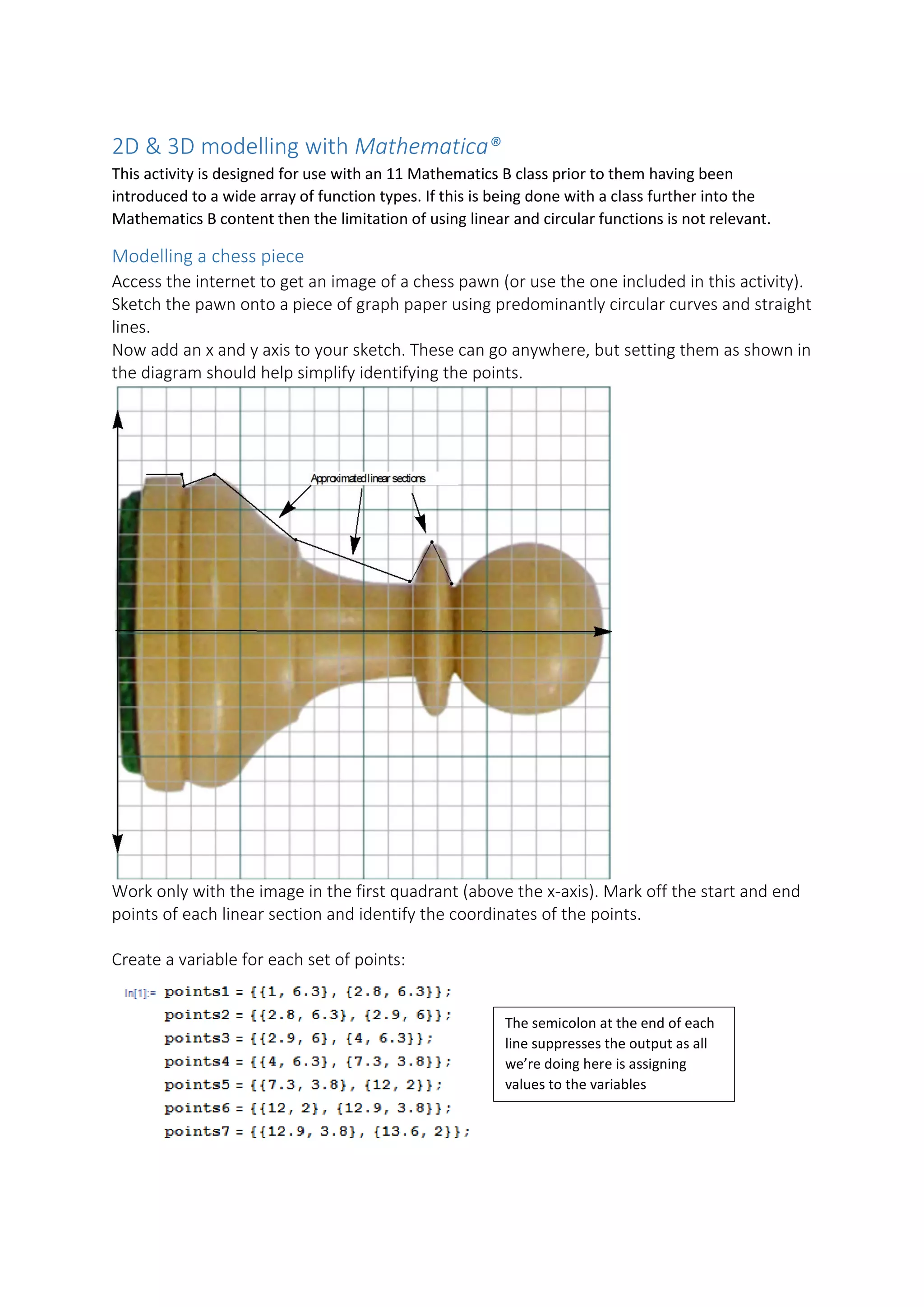
2D & 3D modelling with MathematicaÂŽ
This activity is designed for use with an 11 Mathematics B class prior to them having been
introduced to a wide array of function types. If this is being done with a class further into the
Mathematics B content then the limitation of using linear and circular functions is not relevant.
Modelling a chess piece
Access the internet to get an image of a chess pawn (or use the one included in this activity).
Sketch the pawn onto a piece of graph paper using predominantly circular curves and straight
lines.
Now add an x and y axis to your sketch. These can go anywhere, but setting them as shown in
the diagram should help simplify identifying the points.
Work only with the image in the first quadrant (above the x-axis). Mark off the start and end
points of each linear section and identify the coordinates of the points.
Create a variable for each set of points:
The semicolon at the end of each
line suppresses the output as all
we’re doing here is assigning
values to the variables
Then, determine the equation of each line. For the first segment we can see the equation is
𝑦𝑦 = 6.3 with a domain of (1, 2.8). For the rest of the segments use Mathematica:
For the semicircle section (the head of the pawn) visually identify the centre (h,k) and radius
(r):
Plot the functions with their domains (as specified by the x-values of each set of points). To
restrict a function to the given domain use && - the logical AND construct:
The AspectRatio is set purely for display purposes and is determined from the overall domain
and range indicated on the axes.
You can then repeat this process for the lower half to produce a 2D profile of the pawn, or...
3D plotting
Instead of Plot’ting the functions use RevolutionPlot3D[] on them instead. Here’s a simple
example using the semicircular pawn head:
We could use a semicolon again
as we don’t really need to see
the equations of the functions
at this point if we wished
To display all the functions together on one display use the command Show[] with option
PlotRange -> All. Repeat the RevolutionPlot3D[] command for the rest of the functions to
produce a 3D model of the pawn:
Going further
The code shown here produces a more accurate model of the pawn and can be printed from
a 3D printer. It utilises a broader variety of functions than the original project, such as
exponential and quartic functions. It used a function called NonLinearModelFit[] to
determine the functions for the individual sections. The full mathematical functions have
been included in the code so that it can be copied straight into Mathematica and it will
execute successfully.
To 3D print the design use the Export[] function and export the file as a .stl file.
Using ‘%’ means export the last executed code, so do this as the very next action after having
executed the model producing code.
MathematicaÂŽ is a registered trademark of Wolfram Research, Inc.

2D & 3D Modelling with Mathematica

  • 1.
    2D & 3Dmodelling with Mathematica® This activity is designed for use with an 11 Mathematics B class prior to them having been introduced to a wide array of function types. If this is being done with a class further into the Mathematics B content then the limitation of using linear and circular functions is not relevant. Modelling a chess piece Access the internet to get an image of a chess pawn (or use the one included in this activity). Sketch the pawn onto a piece of graph paper using predominantly circular curves and straight lines. Now add an x and y axis to your sketch. These can go anywhere, but setting them as shown in the diagram should help simplify identifying the points. Work only with the image in the first quadrant (above the x-axis). Mark off the start and end points of each linear section and identify the coordinates of the points. Create a variable for each set of points: The semicolon at the end of each line suppresses the output as all we’re doing here is assigning values to the variables
  • 2.
    Then, determine theequation of each line. For the first segment we can see the equation is 𝑦𝑦 = 6.3 with a domain of (1, 2.8). For the rest of the segments use Mathematica: For the semicircle section (the head of the pawn) visually identify the centre (h,k) and radius (r): Plot the functions with their domains (as specified by the x-values of each set of points). To restrict a function to the given domain use && - the logical AND construct: The AspectRatio is set purely for display purposes and is determined from the overall domain and range indicated on the axes. You can then repeat this process for the lower half to produce a 2D profile of the pawn, or... 3D plotting Instead of Plot’ting the functions use RevolutionPlot3D[] on them instead. Here’s a simple example using the semicircular pawn head: We could use a semicolon again as we don’t really need to see the equations of the functions at this point if we wished
  • 3.
    To display allthe functions together on one display use the command Show[] with option PlotRange -> All. Repeat the RevolutionPlot3D[] command for the rest of the functions to produce a 3D model of the pawn:
  • 4.
    Going further The codeshown here produces a more accurate model of the pawn and can be printed from a 3D printer. It utilises a broader variety of functions than the original project, such as exponential and quartic functions. It used a function called NonLinearModelFit[] to determine the functions for the individual sections. The full mathematical functions have been included in the code so that it can be copied straight into Mathematica and it will execute successfully. To 3D print the design use the Export[] function and export the file as a .stl file. Using ‘%’ means export the last executed code, so do this as the very next action after having executed the model producing code. Mathematica® is a registered trademark of Wolfram Research, Inc.