The document outlines a MATLAB lab exercise focused on function plotting, banded LU factorization, and basic MATLAB commands. It provides detailed instructions for implementing an anonymous function, generating plots, and creating both scripts and function files. Additionally, it introduces MATLAB's environment, command structures, and essential plotting techniques for various mathematical functions.
![2
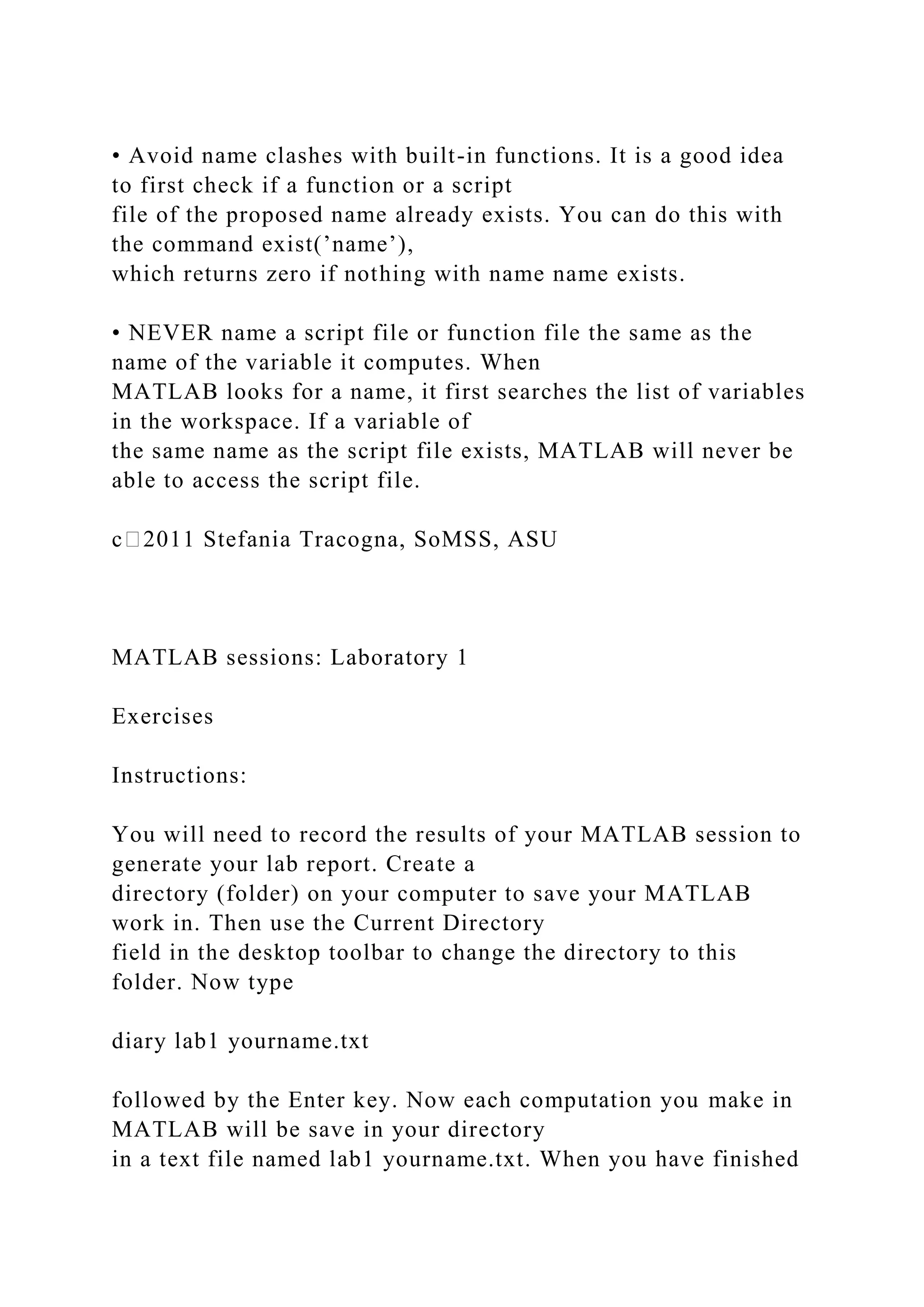
C3 =
3
Joe Bob
Mon lab: 4:30-6:50
Lab 3
Exercise 1
(a) Create function M-file for banded LU factorization
function [L,U] = luband(A,p)
% LUBAND Banded LU factorization
% Adaptation to LUFACT
% Input:
% A diagonally dominant square matrix
% Output:
% L,U unit lower triangular and upper triangular such that
LU=A
n = length(A);
L = eye(n); % ones on diagonal
% Gaussian Elimination](https://image.slidesharecdn.com/samplequestionexercise1considerthefunctionfxc-221112114053-27dbd95b/75/SAMPLE-QUESTIONExercise-1-Consider-the-functionf-x-C-docx-4-2048.jpg)
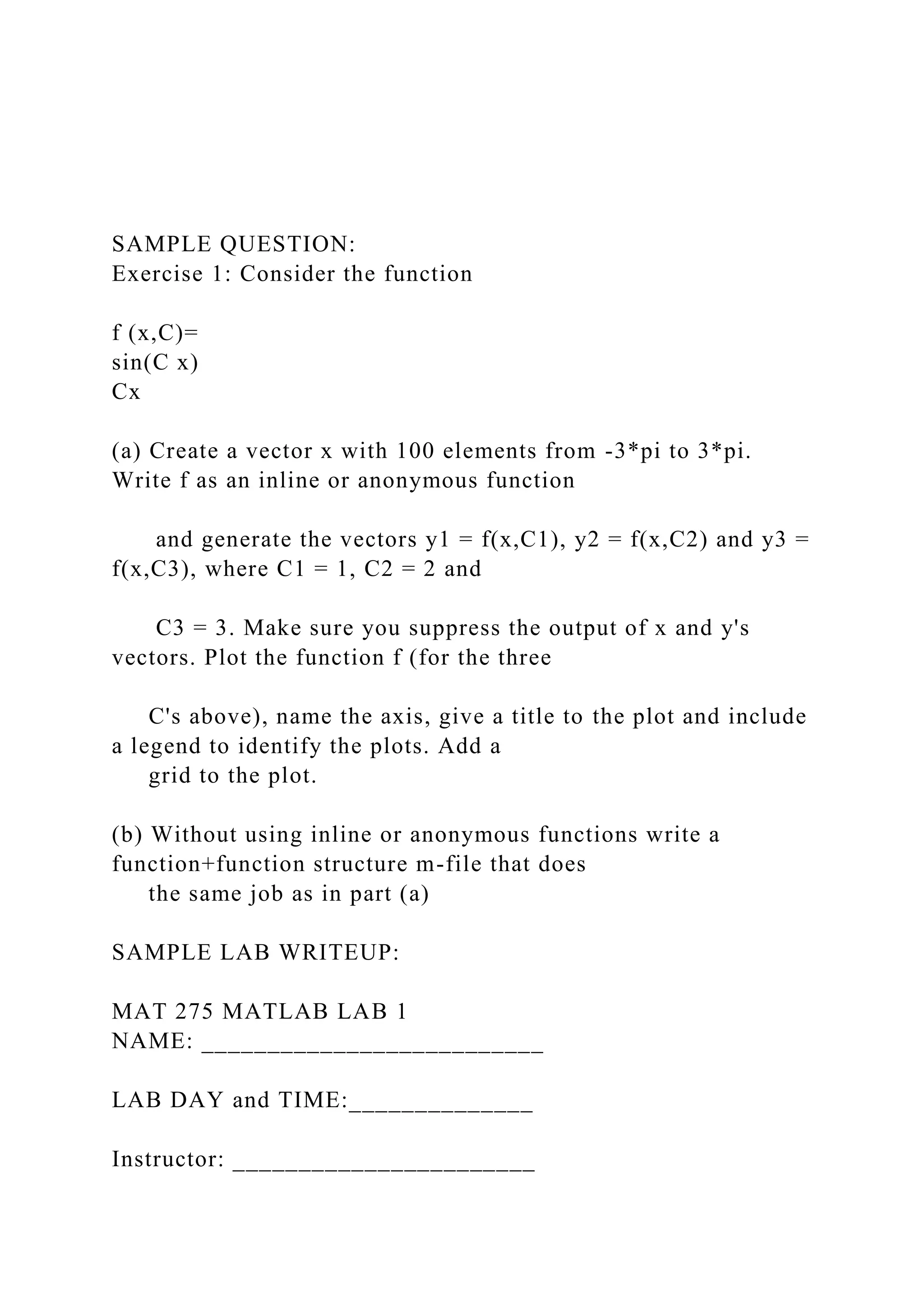
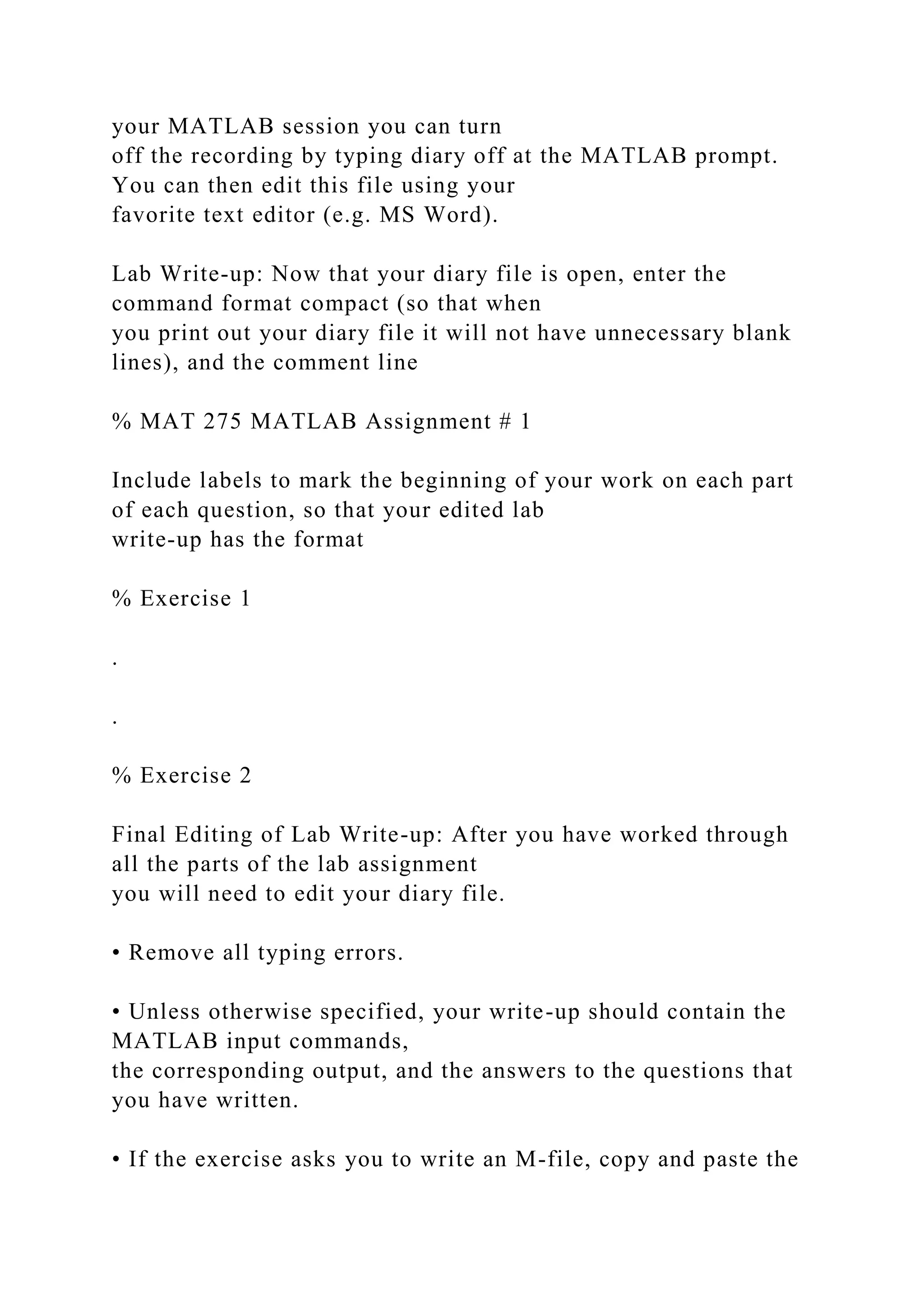
![for j = 1:n-1
a = min(j+p,n);
for i = j+1:a
L(i,j) = A(i,j)/A(j,j); % Row multiplier
b = min(j+p-1,n);
A(i,j:b) = A(i,j:b) - L(i,j)*A(j,j:b);
end
end
U = triu(A);
end
(b) Invoke function in command window
>> A = [1 5 3 -1; 2 4 9 9; 1 1 -1 -3; 4 3 10 3] % declare matrix
A
A =
1 5 3 -1
2 4 9 9
1 1 -1 -3
4 3 10 3
>> luband(A, 4) % call luband function from command window](https://image.slidesharecdn.com/samplequestionexercise1considerthefunctionfxc-221112114053-27dbd95b/75/SAMPLE-QUESTIONExercise-1-Consider-the-functionf-x-C-docx-5-2048.jpg)
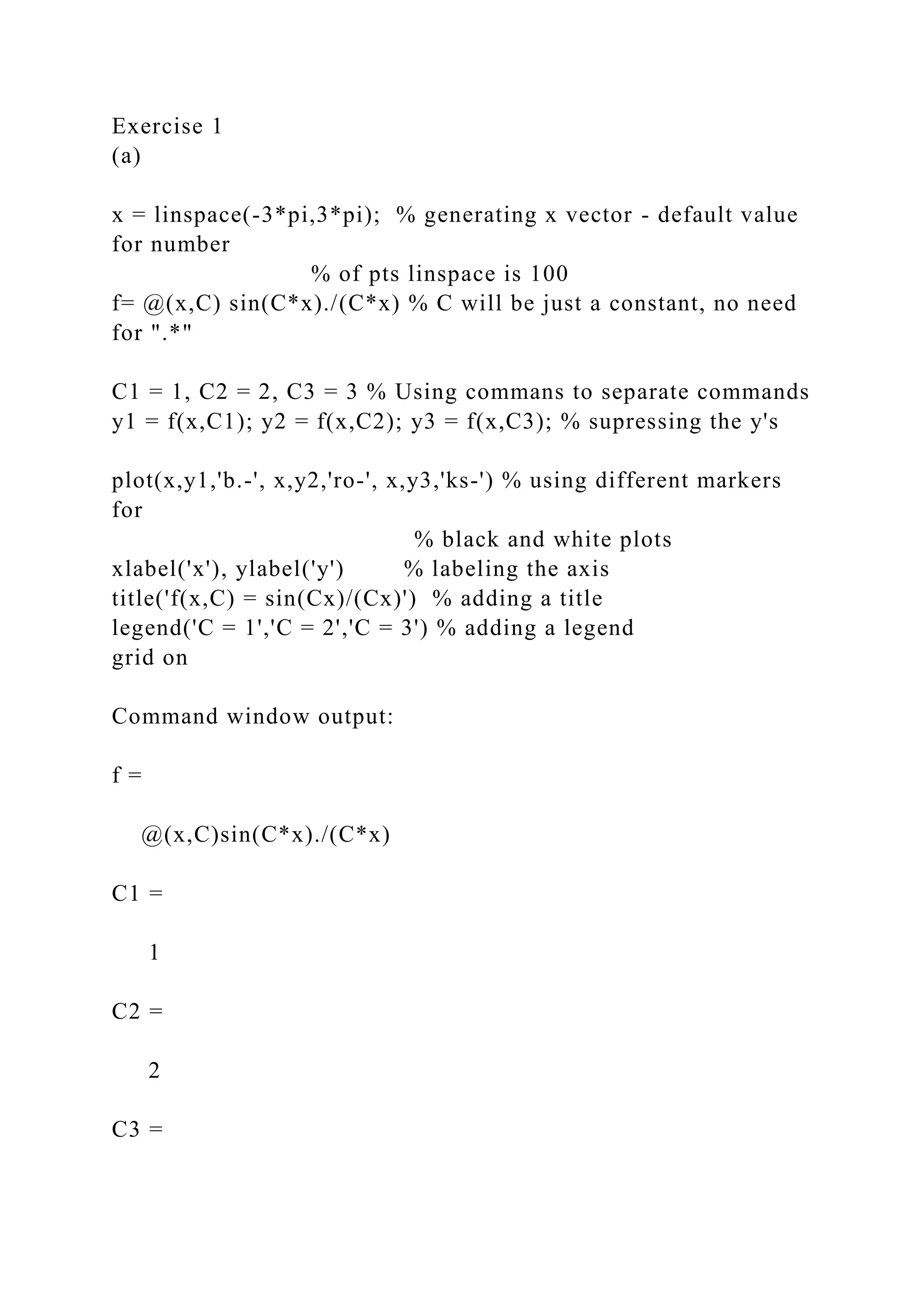
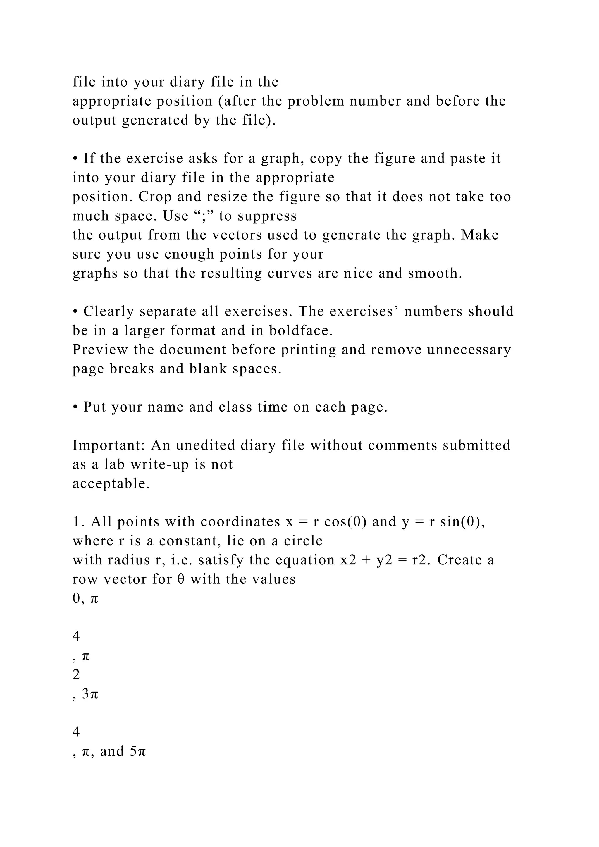
![ans =
1.0000 0 0 0
2.0000 1.0000 0 0
1.0000 0.6667 1.0000 0
4.0000 2.8333 1.7500 1.0000
Exercise 2
(a) Create script-file that runs luband function (Lab3_ex2.m)
A = 10*eye(6)+6*diag(ones(5,1),-1)+6*diag(ones(5,1),1);
[Lband, Uband] = luband(A,2);
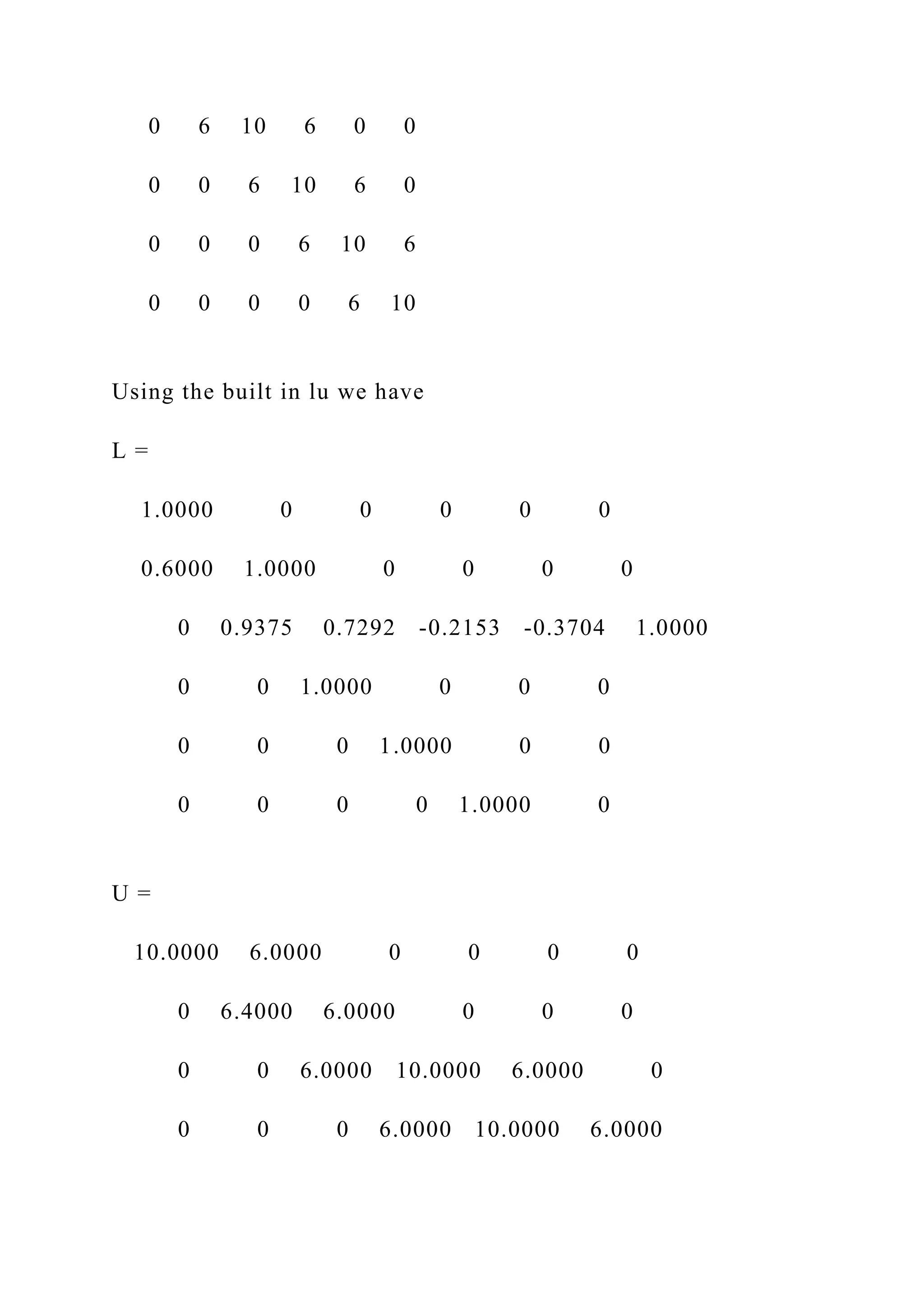
[L, U] = lu(A);
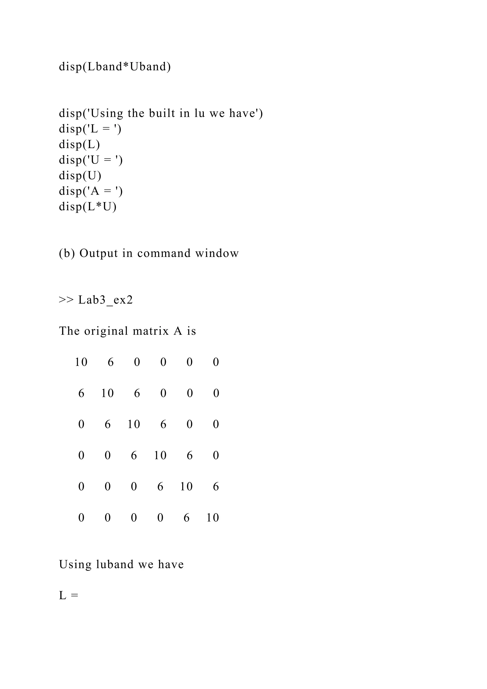
disp('The original matrix A is ')
disp(A)
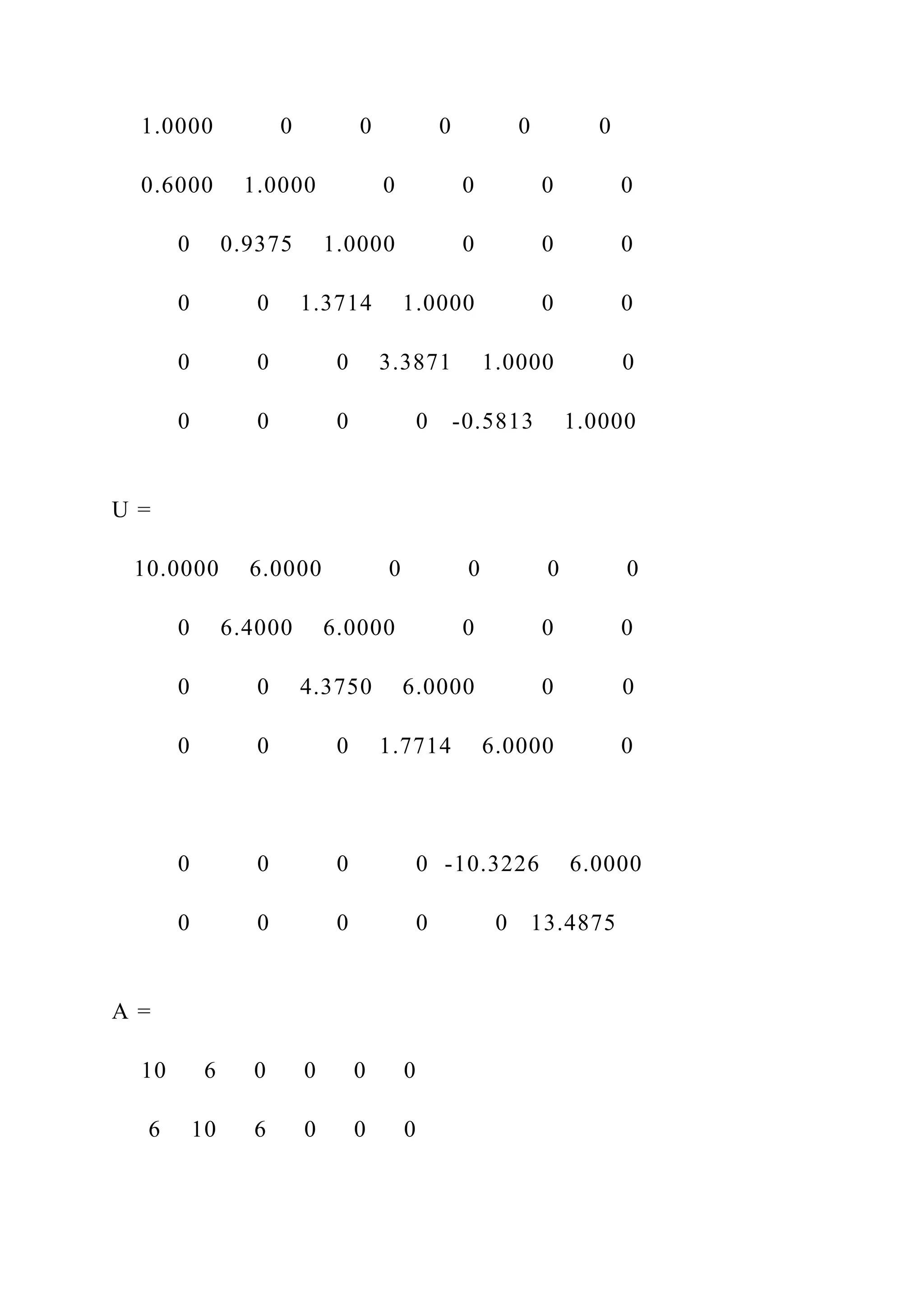
disp('Using luband we have')
disp('L = ')
disp(Lband)
disp('U = ')
disp(Uband)
disp('A = ')](https://image.slidesharecdn.com/samplequestionexercise1considerthefunctionfxc-221112114053-27dbd95b/75/SAMPLE-QUESTIONExercise-1-Consider-the-functionf-x-C-docx-6-2048.jpg)
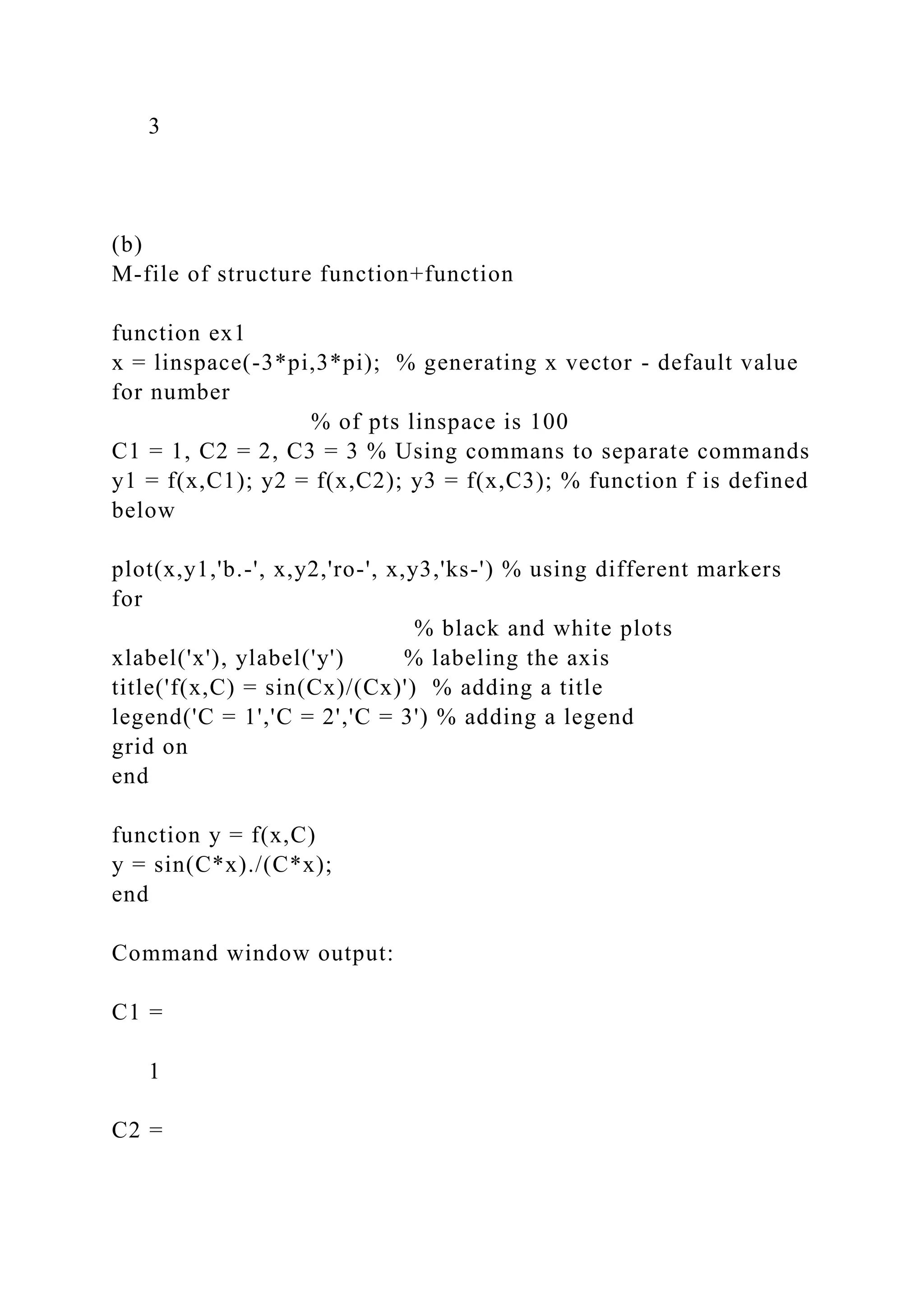
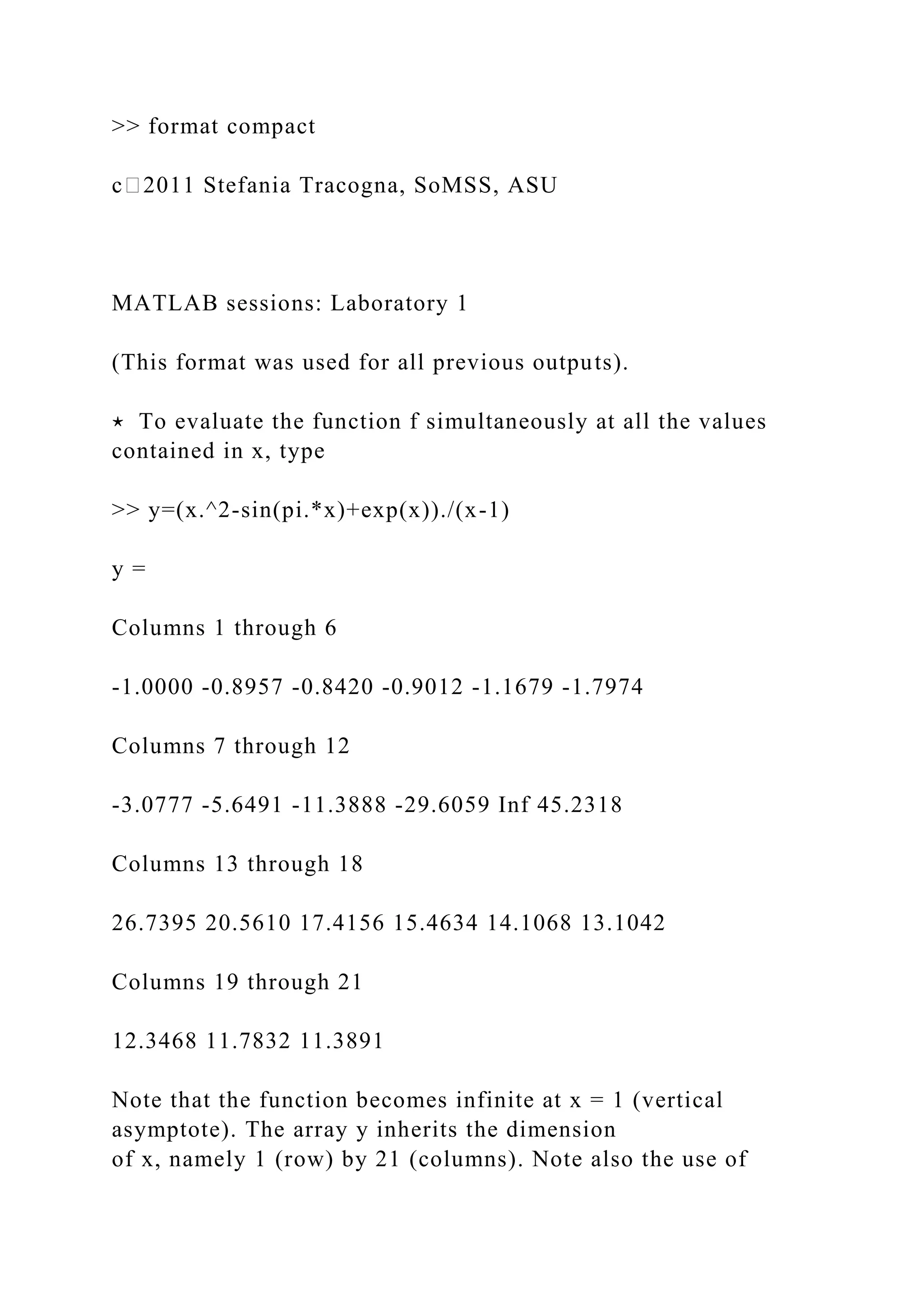
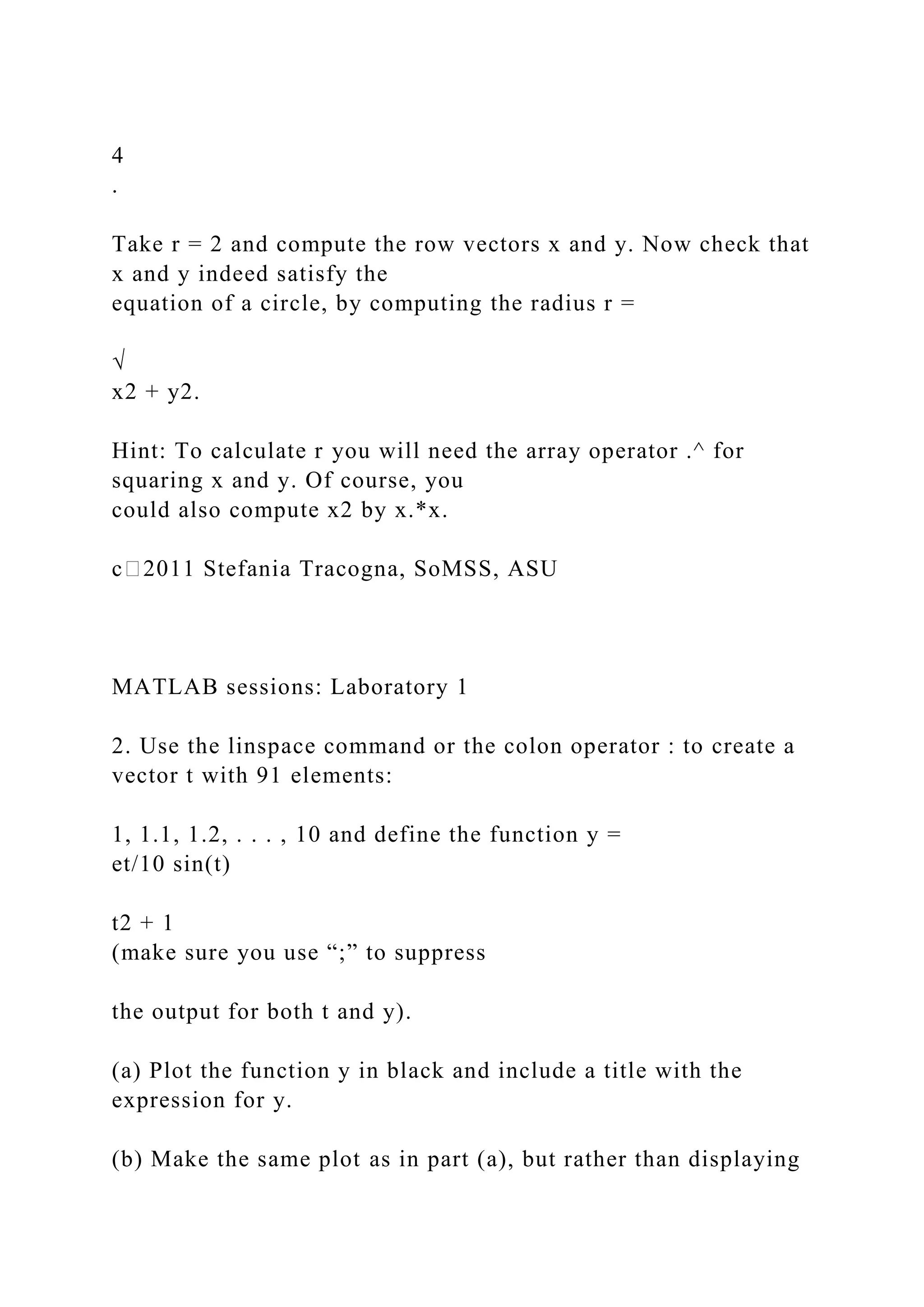
![for 0 ≤ x ≤ 2. First choose a sample of x values in this interval:
>> x=[0,.1,.2,.3,.4,.5,.6,.7,.8,.9,1, ...
1.1,1.2,1.3,1.4,1.5,1.6,1.7,1.8,1.9,2]
x =
Columns 1 through 7
0 0.1000 0.2000 0.3000 0.4000 0.5000 0.6000
Columns 8 through 14
0.7000 0.8000 0.9000 1.0000 1.1000 1.2000 1.3000
Columns 15 through 21
1.4000 1.5000 1.6000 1.7000 1.8000 1.9000 2.0000
Note that an ellipsis ... was used to continue a command too
long to fit in a single line.
Rather than manually entering each entry of the vector x we can
simply use
>> x=0:.1:2
or
>> x=linspace(0,2,21)
Both commands above generate the same output vector x.
⋆ The output for x can be suppressed (by adding ; at the end of
the command) or condensed by entering](https://image.slidesharecdn.com/samplequestionexercise1considerthefunctionfxc-221112114053-27dbd95b/75/SAMPLE-QUESTIONExercise-1-Consider-the-functionf-x-C-docx-15-2048.jpg)
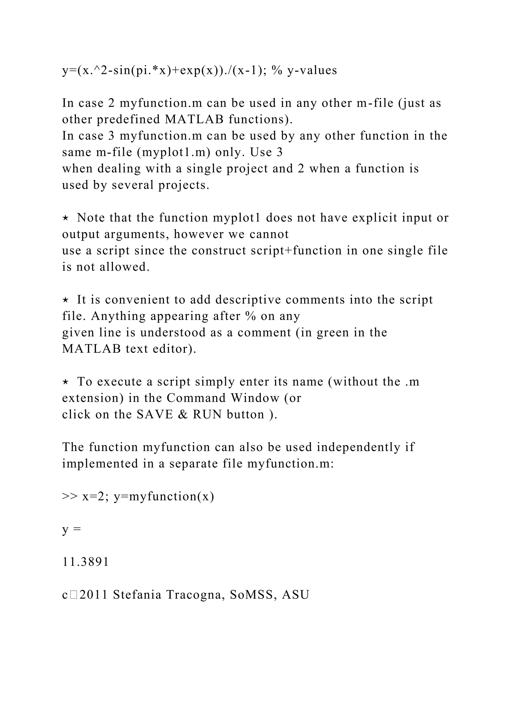
![parentheses.
IMPORTANT REMARK
In the above example *, / and ^ are preceded by a dot . in order
for the expression to be evaluated for
each component (entry) of x. This is necessary to prevent
MATLAB from interpreting these symbols
as standard linear algebra symbols operating on arrays. Because
the standard + and - operations on
arrays already work componentwise, a dot is not necessary for +
and -.
The command
>> plot(x,y)
creates a Figure window and shows the function. The figure can
be edited and manipulated using the
Figure window menus and buttons. Alternately, properties of the
figure can also be defined directly at
the command line:
>> x=0:.01:2;
>> y=(x.^2-sin(pi.*x)+exp(x))./(x-1);
>> plot(x,y,’r-’,’LineWidth’,2);
>> axis([0,2,-10,20]); grid on;
>> title(’f(x)=(x^2-sin(pi x)+e^x)/(x-1)’);
>> xlabel(’x’); ylabel(’y’);
Remarks:](https://image.slidesharecdn.com/samplequestionexercise1considerthefunctionfxc-221112114053-27dbd95b/75/SAMPLE-QUESTIONExercise-1-Consider-the-functionf-x-C-docx-17-2048.jpg)
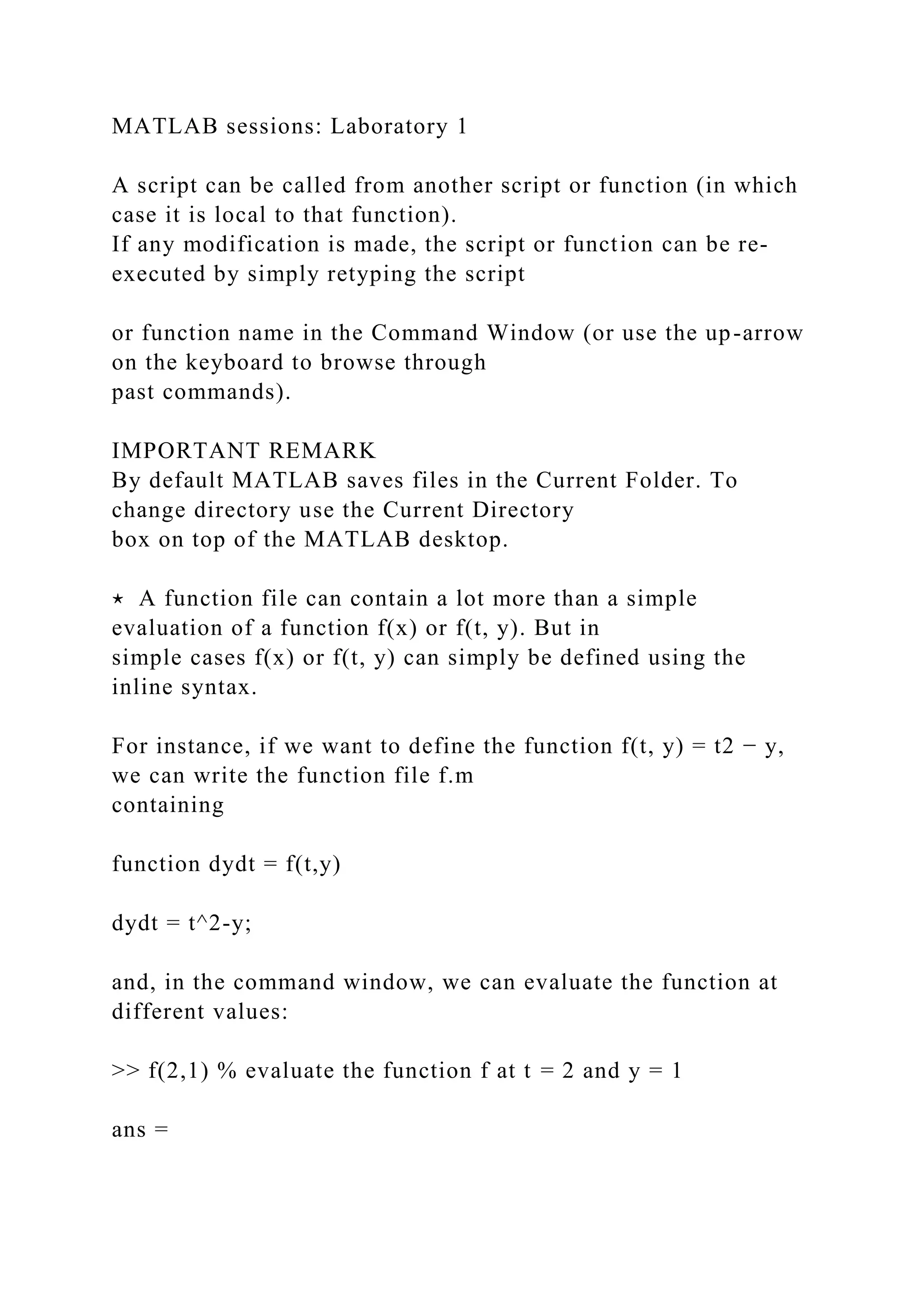
![• The number of x-values has been increased for a smoother
curve (note that the stepsize is now .01
rather than .1).
• The option ’r-’ plots the curve in red.
• ’LineWidth’,2 sets the width of the line to 2 points (the
default is 0.5).
• The range of x and y values has been reset using axis([0,2,-
10,20]) (always a good idea in the
presence of vertical asymptotes).
• The command grid on adds a grid to the plot.
• A title and labels have been added.
The resulting new plot is shown in Fig. L1a. For more options
type help plot in the Command
Window.
c⃝2011 Stefania Tracogna, SoMSS, ASU
MATLAB sessions: Laboratory 1
Figure L1a: A Figure window
Scripts and Functions
⋆ Files containing MATLAB commands are called m-files and
have a .m extension. They are two types:
1. A script is simply a collection of MATLAB commands
gathered in a single file. The value of the](https://image.slidesharecdn.com/samplequestionexercise1considerthefunctionfxc-221112114053-27dbd95b/75/SAMPLE-QUESTIONExercise-1-Consider-the-functionf-x-C-docx-18-2048.jpg)
![data created in a script is still available in the Command
Window after execution. To create a
new script select the MATLAB desktop File menu File > New >
Script. In the MATLAB text
editor window enter the commands as you would in the
Command window. To save the file use
the menu File > Save or File > Save As..., or the shortcut SAVE
button .
Variable defined in a script are accessible from the command
window.
2. A function is similar to a script, but can accept and return
arguments. Unless otherwise specified
any variable inside a function is local to the function and not
available in the command window.
To create a new function select the MATLAB desktop File menu
File > New > Function. A
MATLAB text editor window will open with the following
predefined commands
function [ output_args ] = Untitled3( input_args )
%UNTITLED3 Summary of this function goes here
% Detailed explanation goes here
end
The “output args” are the output arguments, while the “input
args” are the input arguments. The
lines beginning with % are to be replaced with comments
describing what the functions does. The
command(s) defining the function must be inserted after these
comments and before end.
To save the file proceed similarly to the Script M-file.](https://image.slidesharecdn.com/samplequestionexercise1considerthefunctionfxc-221112114053-27dbd95b/75/SAMPLE-QUESTIONExercise-1-Consider-the-functionf-x-C-docx-19-2048.jpg)
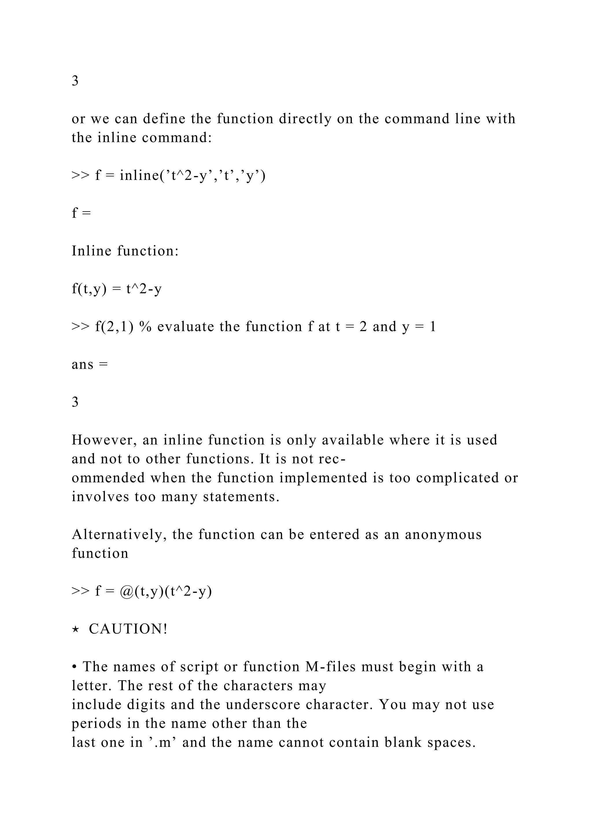
![Use a function when a group of commands needs to be evaluated
multiple times.
⋆ Examples of script/function:
1. script
myplot.m
x=0:.01:2; % x-values
y=(x.^2-sin(pi.*x)+exp(x))./(x-1); % y-values
c⃝2011 Stefania Tracogna, SoMSS, ASU
MATLAB sessions: Laboratory 1
plot(x,y,’r-’,’LineWidth’,2); % plot in red with wider line
axis([0,2,-10,20]); grid on; % set range and add grid
title(’f(x)=(x^2-sin(pi x)+e^x)/(x-1)’); % add title
xlabel(’x’); ylabel(’y’); % add labels
2. script+function (two separate files)
myplot2.m (driver script)
x=0:.01:2; % x-values
y=myfunction(x); % evaluate myfunction at x](https://image.slidesharecdn.com/samplequestionexercise1considerthefunctionfxc-221112114053-27dbd95b/75/SAMPLE-QUESTIONExercise-1-Consider-the-functionf-x-C-docx-20-2048.jpg)
![plot(x,y,’r-’,’LineWidth’,2); % plot in red
axis([0,2,-10,20]); grid on; % set range and add grid
title(’f(x)=(x^2-sin(pi x)+e^x)/(x-1)’); % add title
xlabel(’x’); ylabel(’y’); % add labels
myfunction.m (function)
function y=myfunction(x) % defines function
y=(x.^2-sin(pi.*x)+exp(x))./(x-1); % y-values
3. function+function (one single file)
myplot1.m (driver script converted to function + function)
function myplot1
x=0:.01:2; % x-values
y=myfunction(x); % evaluate myfunction at x
plot(x,y,’r-’,’LineWidth’,2); % plot in red
axis([0,2,-10,20]); grid on; % set range and add grid
title(’f(x)=(x^2-sin(pi x)+e^x)/(x-1)’); % add title
xlabel(’x’); ylabel(’y’); % add labels
%-----------------------------------------
function y=myfunction(x) % defines function](https://image.slidesharecdn.com/samplequestionexercise1considerthefunctionfxc-221112114053-27dbd95b/75/SAMPLE-QUESTIONExercise-1-Consider-the-functionf-x-C-docx-21-2048.jpg)
![dx
= x + 2 is
y(x) =
x2
2
+ 2x + C with y(0) = C.
The goal of this exercise is to write a function file to plot the
solutions to the differential equation
in the interval 0 ≤ x ≤ 4, with initial conditions y(0) = −1, 0, 1.
The function file should have the structure function+function
(similarly to the M-file myplot1.m
Example 3, page 5). The function that defines y(x) must be
included in the same file (note that
the function defining y(x) will have two input arguments: x and
C).
Your M-file should have the following structure (fill in all the
?? with the appropriate commands):
function ex5
x = ?? ; % define the vector x in the interval [0,4]
y1 = f(??); % compute the solution with C = -1
y2 = f(??); % compute the solution with C = 0
y3 = f(??); % compute the solution with C = 1
plot(??) % plot the three solutions with different line-styles
title(??) % add a title](https://image.slidesharecdn.com/samplequestionexercise1considerthefunctionfxc-221112114053-27dbd95b/75/SAMPLE-QUESTIONExercise-1-Consider-the-functionf-x-C-docx-30-2048.jpg)