The document provides a comprehensive overview of edge detection techniques and algorithms used in image processing, including first-order methods (like Roberts, Prewitt, Sobel, and Canny) and second-order methods (like zero-crossing and Marr-Hildreth). It details the steps involved in each method, evaluates their performance, and discusses approaches for motion detection using image differencing and optical flow. Additionally, it includes implementation guidance for these techniques in MATLAB.

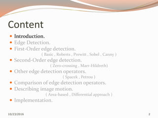
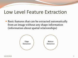
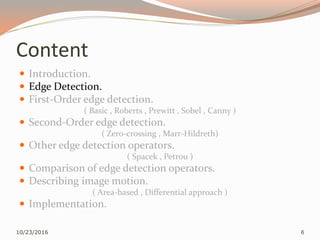
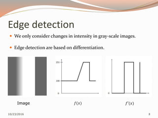
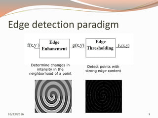
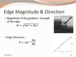
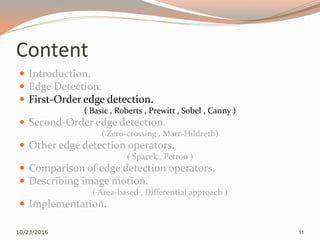
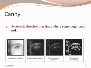
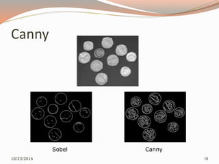
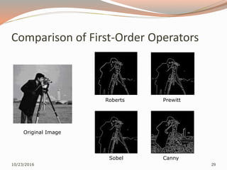
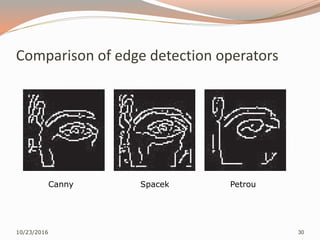
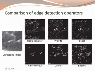
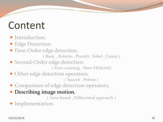
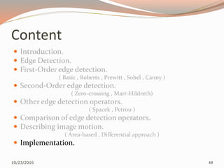
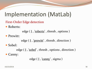
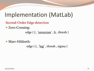
1. By
Alaa Mohammed Khattab
10/23/2016 1

2. Content
 Introduction.
 Edge Detection.
 First-Order edge detection.
( Basic , Roberts , Prewitt , Sobel , Canny )
 Second-Order edge detection.
( Zero-crossing , Marr-Hildreth)
 Other edge detection operators.
( Spacek , Petrou )
 Comparison of edge detection operators.
 Describing image motion.
( Area-based , Differential approach )
 Implementation.
10/23/2016 2

3. Low Level Feature Extraction
10/23/2016 3
Edge
Detection
Motion
Detection
 Basic features that can be extracted automatically
from an image without any shape information
(information about spatial relationships)

4. What is edge ?
Edge defined as change or differences in intensity.
10/23/2016 4

5. Types of edges:
10/23/2016 5
Step (ideal) : Gray values
change suddenly.
Ramp : Grey values
change slowly.

6. Content
 Introduction.
 Edge Detection.
 First-Order edge detection.
( Basic , Roberts , Prewitt , Sobel , Canny )
 Second-Order edge detection.
( Zero-crossing , Marr-Hildreth)
 Other edge detection operators.
( Spacek , Petrou )
 Comparison of edge detection operators.
 Describing image motion.
( Area-based , Differential approach )
 Implementation.
10/23/2016 6

7. Why ?
 Measure the size of the objects in an image.
 Isolate particular objects from their background.
 Recognize or classify objects.
10/23/2016 7

8. Edge detection
 We only consider changes in intensity in gray-scale images.
 Edge detection are based on differentiation.
10/23/2016 8
Image 𝑓(𝑥) 𝑓′(𝑥)

9. Edge detection paradigm
10/23/2016 9
Determine changes in
intensity in the
neighborhood of a point
Detect points with
strong edge content

10. Edge Magnitude & Direction
 Magnitude of the gradient : strength
of the edge.
𝑀 = 𝑀𝑥2 + 𝑀𝑦2
 Edge Direction :
𝜃 = tan−1
𝑀𝑦
𝑀𝑥
10/23/2016 10

11. Content
 Introduction.
 Edge Detection.
 First-Order edge detection.
( Basic , Roberts , Prewitt , Sobel , Canny )
 Second-Order edge detection.
( Zero-crossing , Marr-Hildreth)
 Other edge detection operators.
( Spacek , Petrou )
 Comparison of edge detection operators.
 Describing image motion.
( Area-based , Differential approach )
 Implementation.
10/23/2016 11

12. Basic Operator
 Horizontally
𝐸𝑥 𝑥,𝑦 = |𝑃𝑥,𝑦 − 𝑃𝑥+1,𝑦|
 Vertically
𝐸𝑦𝑥,𝑦 = |𝑃𝑥,𝑦 − 𝑃𝑥,𝑦+1|
 vertical and horizontal edges together
𝐸 𝑥,𝑦 = |2 × 𝑃𝑥,𝑦 − 𝑃𝑥+1,𝑦 − 𝑃𝑥,𝑦+1|
10/23/2016 12

13. Roberts cross 1965
10/23/2016 13
 Two 2×2 templates.
 𝐸𝑥, 𝑦 = max 𝑀+ ∗ 𝑃𝑥, 𝑦 , | 𝑀– ∗ 𝑃𝑥, 𝑦 |

14. Prewitt 1966
10/23/2016 14
 Two 3×3 templates.

15. Sobel 1970
10/23/2016 15
 Two 3×3 templates.
 Can use large templates 5×5 or 7×7.
 larger template involves more smoothing to reduce
noise but edge blurring becomes a great problem.

16. Canny 1986
Canny edge detection is a four step process.
1. Smoothing the image using Gaussian filter (reduce noise
- false edges).
2. Apply Sobel or Perwitt operator.
3. Non-maximum suppression determines if the pixel is
a better candidate for an edge than its neighbors
(thinning).
10/23/2016 16

17. Canny
4. Hysteresis thresholding finds where edges begin and
end.
10/23/2016 17

18. Canny
10/23/2016 18
Sobel Canny

19. Canny
 Good detection – the algorithm should mark as many real
edges in the image as possible.
 Works fine under noisy condition.
 Good localization – edges marked should be as close as
possible to the edge in the real image.
 Minimal response – a given edge in the image should only
be marked once, and where possible, image noise should
not create false edges.
10/23/2016 19

20. Content
 Introduction.
 Edge Detection.
 First-Order edge detection.
( Basic , Roberts , Prewitt , Sobel , Canny )
 Second-Order edge detection.
( Zero-crossing , Marr-Hildreth)
 Other edge detection operators.
( Spacek , Petrou )
 Comparison of edge detection operators.
 Describing image motion.
( Area-based , Differential approach )
 Implementation.
10/23/2016 20

21. Second-Order edge detection
 Zero-crossing of the second derivative of a function
indicates the presence of an edge.
10/23/2016 21

22. Laplacian
10/23/2016 22
The Laplacian operator is a template which implements
second-order differencing.
𝛻2 𝑓 =
𝜕2
𝑓
𝜕𝑥2
+
𝜕2
𝑓
𝜕𝑦2

23. Zero Crossing
10/23/2016 23

24. Marr-Hildreth 1980 (LoG)
1. Smooth the image with a Gaussian filter.
2. Enhance the edges using Laplacian operator.
3. Find the zero-crossing.
10/23/2016 24
Canny LOG

25. Content
 Introduction.
 Edge Detection.
 First-Order edge detection.
( Basic , Roberts , Prewitt , Sobel , Canny )
 Second-Order edge detection.
( Zero-crossing , Marr-Hildreth)
 Other edge detection operators.
( Spacek , Petrou )
 Comparison of edge detection operators.
 Describing image motion.
( Area-based , Differential approach )
 Implementation.
10/23/2016 25

26. Spacek 1986
1. Generate the coefficients of a template-smoothing
operator by:
𝑓 𝑟 = (𝐶1 sin 𝑟 + 𝐶2 cos 𝑟 )𝑒 𝑟
+ (𝐶3 sin 𝑟 + 𝐶4 cos 𝑟 )𝑒−𝑟
+ 1
a circularly symmetric functional expressed in terms of
radius r.
2. Sobel edge detection.
3. Non-maximum suppression.
4. Hysteresis thresholding.
10/23/2016 26

27. Petrou 1991
 Petrou questioned the validity of the step edge model
for real images.
 Any step-changes in the image will be smoothed to
become a ramp.
 Petrou operator uses templates that are 12 pixels wide
at minimum, in order to preserve optimal properties.
10/23/2016 27

28. Content
 Introduction.
 Edge Detection.
 First-Order edge detection.
( Basic , Roberts , Prewitt , Sobel , Canny )
 Second-Order edge detection.
( Zero-crossing , Marr-Hildreth)
 Other edge detection operators.
( Spacek , Petrou )
 Comparison of edge detection operators.
 Describing image motion.
( Area-based , Differential approach )
 Implementation.
10/23/2016 28

29. Comparison of First-Order Operators
10/23/2016 29
Original Image
Roberts Prewitt
Sobel Canny

30. Comparison of edge detection operators
10/23/2016 30
Canny Spacek Petrou

31. Comparison of edge detection operators
10/23/2016 31
Ultrasound image
Basic operator Prewitt Sobel
Marr-Hildreth Canny Spacek

32. Content
 Introduction.
 Edge Detection.
 First-Order edge detection.
( Basic , Roberts , Prewitt , Sobel , Canny )
 Second-Order edge detection.
( Zero-crossing , Marr-Hildreth)
 Other edge detection operators.
( Spacek , Petrou )
 Comparison of edge detection operators.
 Describing image motion.
( Area-based , Differential approach )
 Implementation.
10/23/2016 32

33. Describing image motion
 Motion detection based on comparing of the current
video frame with one from the previous frames.
10/23/2016 33
x
y
time

34. Describing image motion
 The simplest way we can detect motion is by image
differencing.
𝐷 𝑡 = 𝑃 𝑡 − 𝑃(𝑡 − 1)
10/23/2016 34
𝐷 𝑡 = 0
no motion
𝐷 𝑡 ≠ 0
Pixel intensity changes
there is motion

35. 10/23/2016 35
−
=
Second image First image
Difference image

36. Describing image motion
There are a lot of approaches to detect the motion in the
image such as:
 Area-based approach.
 Differential approach.
10/23/2016 36

37. Area-based approach
10/23/2016 37
time t time t+1
(𝑥, 𝑦) ( 𝑥 + 𝛿𝑥 , 𝑦 + 𝛿𝑦 )
Find δx , δy
𝑃(𝑡 + 1) 𝑥+𝛿𝑥 , 𝑦+𝛿𝑦 = 𝑃(𝑡) 𝑥 ,𝑦

38. Area-based approach
 Motion can be characterized as a collection of
displacements in the image plane.
 We try to find correlation between the pixel in the old
and new frames.
10/23/2016 38

39. Area-based approach
 Compare intensities of single pixels:
𝑒 𝑥,𝑦 = ( 𝑃 𝑡 + 1 𝑥+𝛿𝑥 , 𝑦+𝛿𝑦 − 𝑃(𝑡) 𝑥,𝑦 )2
10/23/2016 39

40. Area-based approach
 Consider neighborhood pixels.
𝑒 𝑥,𝑦 =
( 𝑥′,𝑦′)∈𝑊
( 𝑃 𝑡 + 1 𝑥′+𝛿𝑥 , 𝑦′+𝛿𝑦 − 𝑃(𝑡) 𝑥′,𝑦′ )2
10/23/2016 40

41. Area-based approach
Assume that:
 The brightness at the point in the new position should
be the same as the brightness at the old position.
 The neighboring points move with similar velocity.
10/23/2016 41

42. Describing image motion
There are a lot of approaches to detect the motion in the
image such as:
 Area-based approach.
 Differential approach.
10/23/2016 42

43. Differential approach
 Differential techniques compute image velocity from
derivatives of image intensities:
𝑃 𝑥, 𝑦, 𝑡 𝑎𝑛𝑑 𝑃(𝑥 + 𝛿𝑥 , 𝑦 + 𝛿𝑦 , 𝑡 + 𝛿𝑡)
10/23/2016 43

44. Differential approach
Optical Flow:
 The velocity field in the image which transforms
one image into the next image in a sequence.
 Component of optical flow detect the motion
• 𝑢:rate of chang in X
• 𝑣: rate of change in Y
10/23/2016 44

45. Differential approach
 Calculate the 𝑢, v for each pixel.
 Discontinuities in the optical flow can help in
segmenting images into regions that correspond to
different objects.
10/23/2016 45

46. Differential approach
 The pair of equations gives iterative means for calculating
the optical flow of images based on differentials.
𝑢 𝑥,𝑦
𝑛+1 = 𝑢 𝑥,𝑦
𝑛
− λ
𝛻𝑥 𝑥,𝑦 𝑢 𝑥,𝑦 + 𝛻𝑦𝑥,𝑦 𝑣 𝑥,𝑦 + 𝛻𝑡 𝑥,𝑦
1 + λ ( 𝛻𝑥 𝑥,𝑦
2 + 𝛻𝑥 𝑥,𝑦
2)
(𝛻𝑥 𝑥,𝑦 )
𝑣 𝑥,𝑦
𝑛+1
= 𝑣 𝑥,𝑦
𝑛
− λ
𝛻𝑥 𝑥,𝑦 𝑢 𝑥,𝑦 + 𝛻𝑦𝑥,𝑦 𝑣 𝑥,𝑦 + 𝛻𝑡 𝑥,𝑦
1 + λ ( 𝛻𝑥 𝑥,𝑦
2 + 𝛻𝑥 𝑥,𝑦
2)
(𝛻𝑦𝑥,𝑦 )
10/23/2016 46

47. Correlation vs. Differential
Area-based Differential
 Slow.
o high computation.
 Flow is clear.
 Not concerned with rotation.
 Faster than area-based.
 Uncertain flow.
10/23/2016 47

48. Correlation vs. Differential
Area-based Differential
10/23/2016 48

49. Content
 Introduction.
 Edge Detection.
 First-Order edge detection.
( Basic , Roberts , Prewitt , Sobel , Canny )
 Second-Order edge detection.
( Zero-crossing , Marr-Hildreth)
 Other edge detection operators.
( Spacek , Petrou )
 Comparison of edge detection operators.
 Describing image motion.
( Area-based , Differential approach )
 Implementation.
10/23/2016 49

50. Implementation (MatLab)
First-Order Edge detection
 Roberts:
edge ( I , ’roberts’ , thresh , options )
 Prewitt:
edge ( I , ’prewitt’ , thresh , direction )
 Sobel:
edge ( I , ’sobel’ , thresh , options , direction )
 Canny:
edge ( I , ’canny’ , sigma )
10/23/2016 50

51. Implementation (MatLab)
Second-Order Edge detection
 Zero-Crossing:
edge ( I , ’zerocross’ , h , thresh )
 Marr-Hildreth:
edge ( I , ’log’ , thresh , sigma )
10/23/2016 51

52. 10/23/2016 52