The document discusses image processing techniques, focusing on feature detection, description, and matching. It elaborates on various methods such as global vs. local feature representation, Harris corner detection, SIFT, SURF, and LBP, each with its own mechanism for identifying and describing image features. Additionally, it covers feature matching strategies including brute-force and FLANN-based methods to establish correspondences between image features.

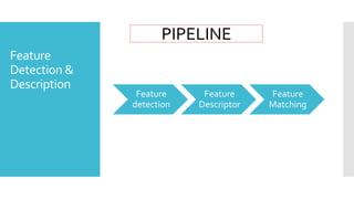
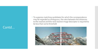
1. IMAGE PROCESSING
&
FEATURE EXTRACTION
By Rishabh Shah

2. Feature
Detection &
Description
Feature
detection
Feature
Descriptor
Feature
Matching
PIPELINE

3. Feature
Detection
The Feature detection are of two types :
1)GLOBAL
2)LOCAL
LOCAL is further divided into three types:
1)SINGLE SCALE
2)Affine Invariant
3)Multi Scale

4. Global vs Local
 Global representation method produces a single vector with
values that measure various aspects of the image such as
color, texture or shape.
 This includes color histograms, texture, edges or even a
specific descriptor extracted from some filters applied to the
image.
 While main goal of local feature representation is to
distinctively represent the image based on some salient
regions while remaining invariant to viewpoint and
illumination changes.
 image is represented based on its local structures by a set of
local feature descriptors extracted from a set of image
regions called interest regions (i.e., keypoints)

5. SingleScale
 Harris corner detection : It basically finds the
difference in intensity for a displacement of in all
directions. This is expressed as below:
 We need to maximize the ‘E’(Intensity of displacement )
and hence we need to maximize the “shifted Intensity”
part of the previous equation. On maximizing we get the
following equation:

6. Contd..
 We get the Eigen values for the equation lambda_1 and
lambda_2. These will help us calculate the score(R):
 If R is small then L1 and L2 both will be small and hence
it indicates flat region.
 If R < 0 , now this when L1>>L2 and hence this detects
the edge .
 If R is large , Now this indicates L1 &L2 are large and
hence the corner is detected.

7. FASTCorner
detection
 FAST(Features from accelerated segment test), In this
method, 16 pixels around the center pixel at a radius r of the
Bresenheim circle are taken. This pixels are further checked
for their intensity values.
 Now the pixel is a corner if there exists a set of contiguous
pixels in the circle (of 16 pixels) which are all brighter than
(Ip + t) or darker then (Ip - t) .

8. Contd..
 Image represents the corner and hence tried to prove the FAST
algorithm.
 Fast is provided with machine learning algorithm ID3 , it is used
to classify the detected points into the classes.
 After a set of key-points are formed non-maximal suppression is
applied. Sometimes adjacent points might turnout to be corner
points and hence to avoid it the lower one is excluded.

9. Hessian
operator
 This operator looks for the points where it’s determinant has a
local maxima.
 Now it looks the points where the derivatives responses are high
in two orthogonal directions.
 Non-Maximum suppression is applied over the pixel values and
hence the maximum among them is carried ahead.
 Then again among all these values the once with intensity values
higher than threshold are taken ahead.
 This all is done because the second order operator is sensitive to
the noise and hence we need the pixel intensities which help in
better description of the image.

10. Multi -Scale
 In multi-scaling part the image key points are identified at various
scales of Gaussian kernel’s scale.
 LoG : LaplacianOf Gaussian, it is a BLOB(Binary LargeObject)
detection method. Now BLOB detection is important because
BLOB tend to represent a set of pixels sharing similar kind of
texture and hence intensity values.
 Operator response is strongly dependent on the relationship
between the size of the blob structures in the image domain and
the size of the smoothing Gaussian kernel. Standard deviation in
Gaussian kernel handles the scaling part.

11. Contd…
 It directly searches for scale invariant features due it’s ability to
find 3D Extrema. It is also circular due to which it is rotation
invariant.

12. Difference of
Gaussian
 DOG- Difference of Gaussian,The DoG function D(x, y,σ) can be
computed without convolution by subtracting adjacent scale
levels of a Gaussian pyramid separated by a factor k.
 We need to select the center pixel and see whether it is greater
than every other pixel around it .

13. GaborWavelet
 The Gabor wavelets are biologically motivated convolution kernels
in the shape of plane waves restricted by a Gaussian envelope
function.
 The advantage of Gabor wavelets is that they provides
simultaneous optimal resolution in both space and spatial
frequency domains.Additionally, Gabor wavelets have the
capability of enhancing low level features such as peaks, valleys
and ridges.
 Sai, represents the wavelet. he coefficients of the convolution,
represent the information in a local image region, which should be
more effective than isolated pixels

14. Feature
Descriptor
 SIFT(Scale Invariant FeatureTransform):
 SCALE SPACE EXTREMA DETECTION: It is nothing but DoG,
hence we further down-sample the image.
 KEYPOINT LOCALIZATION :There are some changes in intensity
values upon changing the brightness and other things and hence
to prevent changes in the keypoints some measures have to be
taken. So we have intensity threshold determined empirically and
similarly we have contrast threshold determined.
We also have hessian matrix for computing the curvature.

15. Contd..
 ORIENTATIONASSIGNMENT:We have to have , the keypoints
invariant to rotation.
 A set of orientation histograms is created where each histogram
contains samples from a 4×4 sub region of the original
neighborhood region and having eight orientations bins in each.
 Hence we have 36 bins of size 10 each (36 X 10 = 360 degrees).
 The peak is the direction of the key point.
 SIFT DESCRIPTOR:The descriptor is then formed from a vector
containing the values of all the orientation histograms entries.
Since there are 4 × 4 histograms each with 8 bins, the feature
vector has 4 × 4 × 8 = 128 elements for each key point

16. SpeededUp
Robust
Features
Detection
(SURF)
 SURF, It uses 2D Box Filter like Hessian Operator unlike SIFT , its
basic idea is to approximate the second order Gaussian derivatives
in an efficient way with the help of integral images using a set of
box filters.
 w is a relative weight for the filter response and it is used to
balance the expression for the Hessian’s determinant.
 The approximated determinant of the Hessian represents the blob
response in the image.
 The SURF descriptor starts by constructing a square region
centered around the detected interest point, and oriented along
its main orientation

17. Contd..
 The interest region is further divided into smaller 4 × 4 sub-regions
and for each sub region the Harr wavelet responses in the vertical
and horizontal directions.
 The wavelet responses dx and dy are summed up for each sub-
region and entered in a feature vector v.
 Computing this for all the 4 × 4 sub-regions, resulting a feature
descriptor of length 4 × 4 × 4 = 64 dimensions.

18. LBP- Local
Binary Pattern
 It characterizes the spatial structure of the texture.
 The LBP feature descriptor:
 LBP has the advantage of tolerance of illumination changes and
computational simplicity.Also, the LBP and its variants achieve
great success in texture description. Unfortunately, the LBP
feature is an index of discrete patterns rather than a numerical
feature.

19. Feature
Matching
 Once the features and their descriptors have been extracted from
two or more images, the next step is to establish some preliminary
feature matches between these images.
 Basics of Brute-Force Matcher
 Brute-Force matcher is simple. It takes the descriptor of one
feature in first set and is matched with all other features in second
set using some distance calculation.And the closest one is
returned.
 FLANN based Matcher
 FLANN stands for Fast Library for Approximate Nearest
Neighbors. It contains a collection of algorithms optimized for fast
nearest neighbor search in large datasets and for high dimensional
features. It works more faster than BFMatcher for large datasets

20. Contd…
 To suppress matching candidates for which the correspondence
may be regarded as ambiguous, the ratio between the distances
to the nearest and the next nearest image descriptor is required to
be less than some threshold

21. THE END.