This document discusses image segmentation, emphasizing techniques for subdividing images into constituent parts, primarily focusing on autonomous segmentation. It outlines key concepts such as discontinuity and similarity in segmentation algorithms, methods for edge detection including the Canny edge detector and the Hough transform, and approaches like thresholding, region growing, and region splitting and merging for processing images. The document details the various methods and challenges in detecting edges, linking and boundary detection, and segmenting regions based on pixel properties.

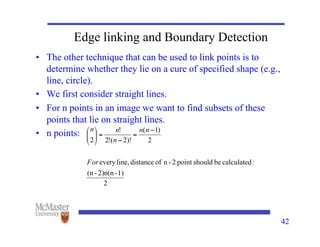
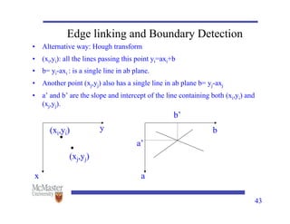
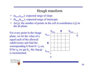
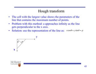
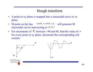
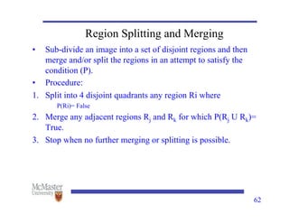
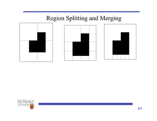
1. CoE4TN4
Image Processing
Chapter 10
Image Segmentation

2. 2
Image Segmentation
• Image analysis: techniques for extracting information from
an image
• The first step in image analysis is to segment the image.
• Segmentation: subdivides the image into its constituent parts
or objects.
• Autonomous segmentation is one of the most difficult tasks
in image processing.
• Segmentation algorithms for monochrome images generally
are based on two basic properties of gray-level values:
1. Discontinuity
2. Similarity

3. 3
Image Segmentation
• Discontinuity: the image is partitioned based on abrupt
changes in gray level
• Similarity: partition an image into regions that are similar
– Main approaches are thresholding, region growing and region splitting
and merging.

4. 4
Detection of Discontinuities
• There are 3 basic types of discontinuities in digital images:
1. Point
2. Line
3. Edges.
• Point detection: detect an isolated point

5. Point Detection
5

6. 6
Background
• Abrupt, local changes can be detected by spatial
differentiation
• Since images are digital we should use digital differentiation
operators.
• First and second order derivatives are commonly used.
• We consider 1-D case first and then expand the results to
images.

7. 7

8. 8
Background
• Comparing first and second order derivatives:
1. First-order derivatives generally produce thicker edges in an
image
2. Second order derivatives have a stronger response to fine
details such as thin lines and isolated points
3. Second order derivates produce a double response at step
changes in gray level

9. 9
Laplacian
• How to obtain 2-D second order derivative and find a mask
corresponding to it?
• We would like our filter to be isotropic: response of the filter
is independent of the direction of the discontinuity in the
image
• Simplest isotropic second order derivative is the Laplacian:

10. Line Detection
10

11. 11
Line Detection
• Line detection: If each mask is moved around an image it
would respond more strongly to lines in the mentioned
direction.

12. 12

13. 13
Edge detection
• Edge: boundary between two regions with relatively distinct
gray levels.
• Basic idea: computation of a local derivative operator.

14. 14
Edge detection
• The magnitude of the first derivative can be used to detect an
edge
• The sign (zero crossing) of the second derivative can be used
to detect an edge.
• The same idea can be extended into 2-D. 2-D derivatives
should be used.
• The magnitude of the gradient and sign of the Laplacian are
used.

15. 15

16. 16
Gradient Operator
• Gradient vector points in the direction of maximum rate of
change of f at (x,y).
Direction of the gradient vector

17. 17
Gradient Operator
• If we compute the magnitude of gradient of an image and
display it, it will be the edges in the image.
• Direction of edge at every point is perpendicular to the
direction of the gradient vector (given by α (x,y)).
• How to approximate the gradient operator?

18. 18

19. 19

20. 20

21. 21

22. 22

23. 23

24. 24
Laplacian of Gaussian
• Laplacian in its original form is not used for edge detection
because:
1. It is very sensitive to noise
2. It’s magnitude produces double edges
3. Unable to detect the direction of an edge.
• To solve the first problem, the image is low-pass filtered
before using the Laplacian operator.
h(x,y)
f(x,y)
g(x,y)

25. 25
Laplacian of Gaussian (LoG)
• Cross section of has a Mexican hat shape.
• The average is zero. The average of image convolved
with is also zero.
• We will have negative pixel values in the result.

26. 26
LoG
• To solve the problem of double edges, zero crossing of the
output of Laplacian operator is used.

27. 27

28. Difference of Gaussian (DoG)
• LoG can be approximated by a difference of Gaussians:
28
DoG(x, y) =
1
2⇡ 2
1
e
x2+y2
2 2
1
1
2⇡ 2
2
e
x2+y2
2 2
2
2
=
2
1
2
2
2
1
2
2
ln
2
1
2
2

29. 29

30. Canny edge detector
• 1) Low error rate. All edges should be found, and there should
be no spurious responses.
• 2) Edge points should be well localized. The edges must be as
close as possible to true edges.
• 3) Single edge point response. The detector should not
identify multiple edge pixels where only a single edge point
exist
30

31. Canny edge detector
• Input image f(x,y) is smoothed using a Gaussian filter and
then the gradient magnitude and direction are calculated
31
G(x, y) = e
x2+y2
2 2
fs(x, y) = G(x, y) ? f(x, y)
M(x, y) =
q
g2
x + g2
y
↵(x, y) = arctan
gy
gx

32. Canny edge detector
• M(x,y) typically contains wide ridges around local maxima
• Thinning those ridges: nonmaxima suppression
• Let d1,d2,d3 and d4 denote the 4 basic edge directions.
• In every 3x3-region:
– Find the direction dk that is closest to α(x,y).
– If the value of M(x,y) is less than one of its two neighbors along dk,
suppress edge.
32

33. Canny edge detector
33

34. Canny edge detector
• Final step: reduce false edge points.
• Reduce them using hysteresis (or double) thresholding.
• Let 𝑇𝐿 ,𝑇𝐻 be low and high thresholds. The suggested ratio is
𝐿 ,𝑇𝐻 be low and high thresholds. The suggested ratio is
,𝑇𝐻 be low and high thresholds. The suggested ratio is
𝐻 be low and high thresholds. The suggested ratio is
be low and high thresholds. The suggested ratio is
1:3 or 2:3.
• Define 𝑔𝑁𝐻(𝑥,𝑦) and 𝑔𝑁𝐿(𝑥,𝑦) to be 𝑔𝑁(𝑥,𝑦) after thresholding
𝑁𝐻(𝑥,𝑦) and 𝑔𝑁𝐿(𝑥,𝑦) to be 𝑔𝑁(𝑥,𝑦) after thresholding
(𝑥,𝑦) and 𝑔𝑁𝐿(𝑥,𝑦) to be 𝑔𝑁(𝑥,𝑦) after thresholding
) and 𝑔𝑁𝐿(𝑥,𝑦) to be 𝑔𝑁(𝑥,𝑦) after thresholding
𝑁𝐿(𝑥,𝑦) to be 𝑔𝑁(𝑥,𝑦) after thresholding
(𝑥,𝑦) to be 𝑔𝑁(𝑥,𝑦) after thresholding
) to be 𝑔𝑁(𝑥,𝑦) after thresholding
𝑁(𝑥,𝑦) after thresholding
(𝑥,𝑦) after thresholding
) after thresholding
with 𝑇𝐿 ,𝑇𝐻.
𝐿 ,𝑇𝐻.
,𝑇𝐻.
𝐻.
.
• It is clear that 𝑔𝑁𝐿(𝑥,𝑦) contains all the point located in
𝑁𝐿(𝑥,𝑦) contains all the point located in
(𝑥,𝑦) contains all the point located in
) contains all the point located in
𝑔𝑁𝐻(𝑥,𝑦)
𝑁𝐻(𝑥,𝑦)
(𝑥,𝑦)
)
• We will separate them by subtraction: 𝑔𝑁𝐿(𝑥,𝑦)= 𝑔𝑁𝐻(𝑥,𝑦) −
𝑁𝐿(𝑥,𝑦)= 𝑔𝑁𝐻(𝑥,𝑦) −
(𝑥,𝑦)= 𝑔𝑁𝐻(𝑥,𝑦) −
)= 𝑔𝑁𝐻(𝑥,𝑦) −
𝑁𝐻(𝑥,𝑦) −
(𝑥,𝑦) −
) −
𝑔𝑁𝐿(𝑥,𝑦)
𝑁𝐿(𝑥,𝑦)
(𝑥,𝑦)
)
• Now 𝑔𝑁𝐿(𝑥,𝑦) and 𝑔𝑁𝐻(𝑥,𝑦) are the “weak” and the “strong”
𝑁𝐿(𝑥,𝑦) and 𝑔𝑁𝐻(𝑥,𝑦) are the “weak” and the “strong”
(𝑥,𝑦) and 𝑔𝑁𝐻(𝑥,𝑦) are the “weak” and the “strong”
) and 𝑔𝑁𝐻(𝑥,𝑦) are the “weak” and the “strong”
𝑁𝐻(𝑥,𝑦) are the “weak” and the “strong”
(𝑥,𝑦) are the “weak” and the “strong”
) are the “weak” and the “strong”
edge pixels.
34

35. Canny edge detector
• The algorithm for building the edges is:
• 1. Locate the next unvisited pixel 𝑝 in 𝑔𝑁𝐻(𝑥,𝑦).
in 𝑔𝑁𝐻(𝑥,𝑦).
𝑁𝐻(𝑥,𝑦).
(𝑥,𝑦).
).
• 2. Mark as valid pixels all the weak pixels in 𝑔𝑁𝐿(𝑥,𝑦) that are
𝑁𝐿(𝑥,𝑦) that are
(𝑥,𝑦) that are
) that are
connected to 𝑝
• 3. If not all non-zero pixels in 𝑔𝑁𝐻(𝑥,𝑦) have been visited
𝑁𝐻(𝑥,𝑦) have been visited
(𝑥,𝑦) have been visited
) have been visited
return to step 1.
• 4. Set all the non-marked pixels in 𝑔𝑁𝐿(𝑥,𝑦) to 0.
𝑁𝐿(𝑥,𝑦) to 0.
(𝑥,𝑦) to 0.
) to 0.
• 5. Return 𝑔𝑁𝐻(𝑥,𝑦) + 𝑔𝑁𝐿(𝑥,𝑦).
𝑁𝐻(𝑥,𝑦) + 𝑔𝑁𝐿(𝑥,𝑦).
(𝑥,𝑦) + 𝑔𝑁𝐿(𝑥,𝑦).
) + 𝑔𝑁𝐿(𝑥,𝑦).
𝑁𝐿(𝑥,𝑦).
(𝑥,𝑦).
).
35

36. Canny edge detector
36

37. 37
Edge linking and Boundary Detection
• The output of discontinuity detection stage seldom
characterizes a boundary completely.
• This is because of noise, breaks in the boundary and other
effects.
• Edge detection algorithms typically are followed by linking
and boundary detection procedures.
• These procedures assemble edge pixels into meaningful
boundaries.

38. 38
Edge linking and Boundary Detection
• A simple approach for linking edge points is to analyze the
pixels in a small neighborhood about every point (x,y).
• All the points that are similar are linked forming a boundary
of pixels.
• Two principle properties used for establishing similarity of
edge pixels in this kind of analysis are:
1. The strength of the response of the gradient operator used to produce
the edge pixels
2. The direction of the gradient
|M(s, t) M(x, y)|  E
|↵(s, t) ↵(x, y)|  A

39. Local Processing
• 1.Compute the gradient magnitude and angle arrays, M(x,y)
and α(x,y), of the input image, f(x,y) .
• 2.Form a binary image, g, whose value at any pair of
coordinates (x,y) is given by:
• where TM is a threshold, A is a specified angle direction, and
±TA defines a “band” of acceptable directions about A
39

40. Local Processing
• 3. Scan the rows of g and fill (set to 1) all gaps (sets of 0s) in
each row that do not exceed a specified length, K. Note that,
by definition, a gap is bounded at both ends by one or more
1s. The rows are processed individually with no memory
between them.
• 4. To detect gaps in any other direction, θ, rotate g by this
angle and apply the horizontal scanning procedure in step 3.
Rotate the result back by -θ.
40

41. 41
Edge linking and Boundary Detection

42. 42
Edge linking and Boundary Detection
• The other technique that can be used to link points is to
determine whether they lie on a cure of specified shape (e.g.,
line, circle).
• We first consider straight lines.
• For n points in an image we want to find subsets of these
points that lie on straight lines.
• n points:

43. 43
Edge linking and Boundary Detection
• Alternative way: Hough transform
• (xi,yi): all the lines passing this point yi=axi+b
• b= yi-axi : is a single line in ab plane.
• Another point (xj,yj) also has a single line in ab plane b= yj-axj
• a’ and b’ are the slope and intercept of the line containing both (xi,yi) and
(xj,yj).
(xi,yi)
(xj,yj)
x
y
a
b
a’
b’

44. 44
Hough transform
• (amin,amax): expected range of slope
• (bmin,bmax): expected range of intercepts
• A(i,j): the number of points in the cell at coordinates (i,j) in
the ab plane.
amin
amax
bmin bmax
0
0
a
b
For every point in the image
plane, we let the value of a
equal each of the allowed
subdivisions and find the
corresponding b from b= yi-axi
If for ap we get bq the A(p,q)
is incremented.

45. 45
Hough transform
• The cell with the largest value shows the parameters of the
line that contains the maximum number of points.
• Problem with this method: a approaches infinity as the line
gets perpendicular to the x axis.
• Solution: use the representation of the line as:
y
x

46. 46
Hough transform
• A point in xy plane is mapped into a sinusoidal curve in
plane.
• M point on the line will generate M
sinusoidal curves intersecting at
• For increments of between –90 and 90, find the value of
for every point in xy plane. Increment the corresponding cell
counter.
y
x

47. 47

48. 48
Hough transform
• Hough transform is applicable to any function of the form g(v,c)=0,
where v is the vector of coordinates and c is the vector of coefficients.
• Exp:
• 3 parameters (c1,c2,c3), 3-D parameter space, cube like cells,
accumulators of the form A(i,j,k).
• Procedure:
1. Increment c1 and c2
2. Solve for c3
3. Update the accumulator associated with (c1,c2,c3)

49. 49

50. 50
Thresholding
• Thresholding is one of the most important approaches to
image segmentation.
• Gray level histogram of an image f(x,y) composed of a
light object on a dark background.
• To extract the object: select a threshold T that separates
the gray levels of the background and the object.
• Any point with f(x,y)>T belongs to object.

51. 51
Thresholding

52. 52

53. 53
Thresholding
• Threshold in general can be calculated as:
T=T(x,y,p(x,y),f(x,y))
f(x,y): gray level at (x,y)
p(x,y): some local property of the point (x,y) (e.g., the average gray level
of a neighborhood centered on (x,y).
T depends only on f(x,y): global threshold
T depends on f(x,y) and p(x,y): local threshold
T depends on f(x,y) and p(x,y) and x,y : dynamic threshold

54. 54
Thresholding
• Poor or non-uniform illumination can affect the image formed
(because of f(x,y)=r(x,y).i(x,y)) and make the segmentation
difficult.
• Solution: if we can determine i(x,y) then we can compensate f
for the effects of i.
• Technique: Project the illumination source onto a constant,
white reflective surface. The image obtained is
g(x,y)=K.i(x,y) (K is a constant).
• Divide f(x,y) by g(x,y): h(x,y)=f(x,y)/g(x,y)=r(x,y)/K
• If r(x,y) can be segmented by thresholding, then h(x,y) can
also be segmented by thresholding.

55. 55
Thresholding
• How to find a proper value for T?
1. Select an initial estimate for T
2. Segment the image using T. This will produce two group of
pixels G1 (with gray level greater than T) and G2 (with gray
level less than T)
3. Compute average gray level values µ1 and µ2 for pixels in
regions G1 and G2
4. Compute a new threshold: T=(µ1+ µ2)/2
5. Repeat step 2 through 4 until the difference in T in
successive iterations is smaller than a predefined value

56. Optimal Global Thresholding (Otsu’s method)
• The method is optimum in the sense that it maximizes the
between-class variance, a well-known measure used in the
statistical discriminant analysis.
• Well-thresholded classes should be distinct with respect to the
intensity values of their pixels
56

57. Otsu’s method
• Improve the histogram shape by considering only those pixels
laying on or near the edges between objects and the
backgrounds
• Histogram would be less dependent on the relative sizes of
objects and backgrounds
• Using pixels that satisfy some simple measures based on the
gradient and Laplacian operators has a tendency to deepen the
valley between histogram peaks (i.e., pixels are selected by a
gradient/Laplacian criterion)
57

58. Otsu’s method
58

59. 59
Region Based Segmentation
• Let R represent the entire image. Segmentation is a process
that partitions R into n subregions R1,R2,…,Rn such that:

60. 60
Region growing by Pixel Aggregation
• Pixel aggregation: starts with a set of seed point and from
these grows regions by appending to each seed point those
neighboring pixels that have similar properties (e.g., gray-
level, texture, color).
0 0 5 6 7
1 1 5 8 7
0 1 6 7 7
2 0 7 6 6
0 1 5 6 5
A A B B B
A A B B B
A A B B B
A A B B B
A A B B B
T=3

61. 61
Region growing by Pixel Aggregation
• Problems:
1. Selection of initial seeds that properly represent regions of interest
2. Selection of suitable properties
3. Formulation of a stopping rule.

62. 62
Region Splitting and Merging
• Sub-divide an image into a set of disjoint regions and then
merge and/or split the regions in an attempt to satisfy the
condition (P).
• Procedure:
1. Split into 4 disjoint quadrants any region Ri where
P(Ri)= False
2. Merge any adjacent regions Rj and Rk for which P(Rj U Rk)=
True.
3. Stop when no further merging or splitting is possible.

63. 63
Region Splitting and Merging