Downloaded 143 times


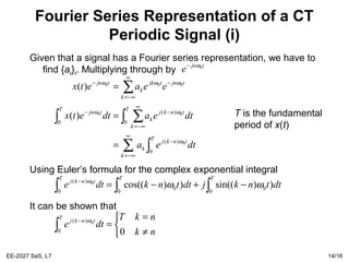
![EE-2027 SaS, L7 15/16
Fourier Series Representation of a CT
Periodic Signal (ii)
Therefore
which allows us to determine the coefficients. Also note that this
result is the same if we integrate over any interval of length T
(not just [0,T]), denoted by
To summarise, if x(t) has a Fourier series representation, then the
pair of equations that defines the Fourier series of a periodic,
continuous-time signal:
∫
−
=
T
tjn
Tn dtetxa
0
1 0
)( ω
∫T
∫
−
=
T
tjn
Tn dtetxa 0
)(1 ω
∫∫
∑∑
−−
∞
−∞=
∞
−∞=
==
==
T
tTjk
TT
tjk
Tk
k
tTjk
k
k
tjk
k
dtetxdtetxa
eaeatx
)/2(11
)/2(
)()(
)(
0
0
πω
πω](https://image.slidesharecdn.com/lecture6-131002071533-phpapp02/85/Lecture6-Signal-and-Systems-15-320.jpg)


This document summarizes a lecture on Fourier series and basis functions. It introduces Fourier series representation of periodic time functions using a basis of complex exponentials. A periodic signal can be expressed as a sum of these basis functions multiplied by coefficients. The coefficients can be determined by integrating the signal multiplied by basis functions over one period. Complex exponentials are eigenfunctions of linear time-invariant systems, and the corresponding eigenvalues can be used to determine the output of such systems when the input is an eigenfunction.