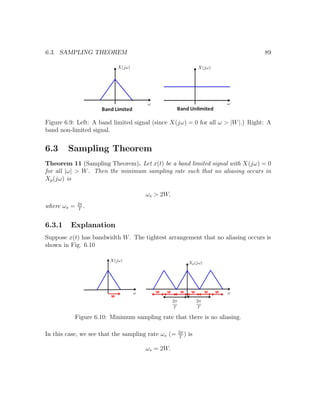
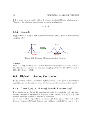
This document is a class note for a signals and systems course. It was prepared by Stanley Chan at UC San Diego in 2011 using notes from Prof. Paul H. Siegel. The note covers topics in signals and systems including fundamentals of signals, systems, Fourier series, continuous-time Fourier transform, discrete-time Fourier transform, sampling theorem, and z-transform. It contains examples and definitions for key concepts. The textbook used for the course is Signals and Systems by Oppenheim and Wilsky.
![Chapter 1
Fundamentals of Signals
1.1 What is a Signal?
A signal is a quantitative description of a physical phenomenon, event or process.
Some common examples include:
1. Electrical current or voltage in a circuit.
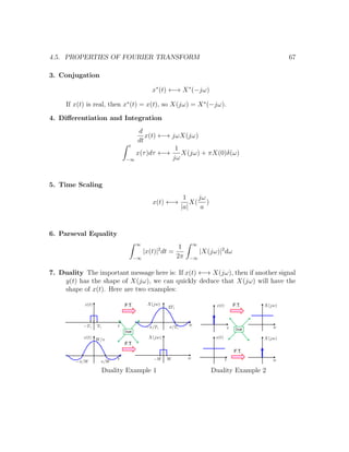
2. Daily closing value of a share of stock last week.
3. Audio signal: continuous-time in its original form, or discrete-time when stored
on a CD.
More precisely, a signal is a function, usually of one variable in time. However, in
general, signals can be functions of more than one variable, e.g., image signals.
In this class we are interested in two types of signals:
1. Continuous-time signal x(t), where t is a real-valued variable denoting time,
i.e., t ∈ R. We use parenthesis (·) to denote a continuous-time signal.
2. Discrete-time signal x[n], where n is an integer-valued variable denoting the
discrete samples of time, i.e., n ∈ Z. We use square brackets [·] to denote a
discrete-time signal. Under the definition of a discrete-time signal, x[1.5] is not
defined, for example.
5](https://image.slidesharecdn.com/note0-160519103024/85/Note-0-5-320.jpg)
![6 CHAPTER 1. FUNDAMENTALS OF SIGNALS
1.2 Review on Complex Numbers
We are interested in the general complex signals:
x(t) ∈ C and x[n] ∈ C,
where the set of complex numbers is defined as
C = {z | z = x + jy, x, y ∈ R, j =
√
−1.}
A complex number z can be represented in Cartesian form as
z = x + jy,
or in polar form as
z = rejθ
.
Theorem 1. Euler’s Formula
ejθ
= cos θ + j sin θ. (1.1)
Using Euler’s formula, the relation between x, y, r, and θ is given by
x = r cos θ
y = r sin θ
and
r = x2 + y2,
θ = tan−1 y
x
.
Figure 1.1: A complex number z can be expressed in its Cartesian form z = x + jy, or in its polar
form z = rejθ
.](https://image.slidesharecdn.com/note0-160519103024/85/Note-0-6-320.jpg)
![1.3. BASIC OPERATIONS OF SIGNALS 7
A complex number can be drawn on the complex plane as shown in Fig. 1.1. The
y-axis of the complex plane is known as the imaginary axis, and the x-axis of the
complex plane is known as the real axis. A complex number is uniquely defined by
z = x + jy in the Cartesian form, or z = rejθ
in the polar form.
Example. Convert the following complex numbers from Cartesian form to polar
form: (a) 1 + 2j; (b) 1 − j.
For (a), we apply Euler’s formula and find that
r =
√
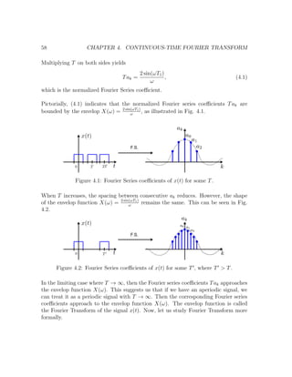
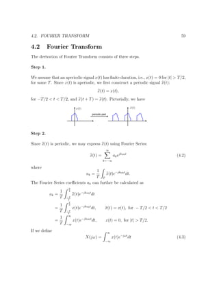
12 + 22 =
√
5, and θ = tan−1 2
1
≈ 63.64◦
.
Therefore,
1 + 2j =
√
5ej63.64◦
.
For (b), we apply Euler’s formula again and find that
r = 12 + (−1)2 =
√
2, and θ = tan−1 −1
1
= −45◦
.
Therefore,
1 − j =
√
2e−jπ/4
.
Recall that: π in radian = 180◦
in degree.
Example. Calculate the value of jj
.
jj
= (ejπ/2
)j
= e−π/2
≈ 0.2078.
1.3 Basic Operations of Signals
1.3.1 Time Shift
For any t0 ∈ R and n0 ∈ Z, time shift is an operation defined as
x(t) −→ x(t − t0)
x[n] −→ x[n − n0].
(1.2)
If t0 > 0, the time shift is known as “delay”. If t0 < 0, the time shift is known as
“advance”.
Example. In Fig. 1.2, the left image shows a continuous-time signal x(t). A time-
shifted version x(t − 2) is shown in the right image.](https://image.slidesharecdn.com/note0-160519103024/85/Note-0-7-320.jpg)
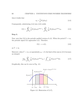
![8 CHAPTER 1. FUNDAMENTALS OF SIGNALS
Figure 1.2: An example of time shift.
1.3.2 Time Reversal
Time reversal is defined as
x(t) −→ x(−t)
x[n] −→ x[−n],
(1.3)
which can be interpreted as the “flip over the y-axis”.
Example.
Figure 1.3: An example of time reversal.
1.3.3 Time Scaling
Time scaling is the operation where the time variable t is multiplied by a constant a:
x(t) −→ x(at), a > 0 (1.4)
If a > 1, the time scale of the resultant signal is “decimated” (speed up). If 0 < a < 1,
the time scale of the resultant signal is “expanded” (slowed down).
1.3.4 Combination of Operations
In general, linear operation (in time) on a signal x(t) can be expressed as y(t) = x(at−
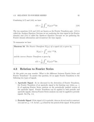
b), a, b ∈ R. There are two methods to describe the output signal y(t) = x(at − b).](https://image.slidesharecdn.com/note0-160519103024/85/Note-0-8-320.jpg)
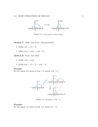
![10 CHAPTER 1. FUNDAMENTALS OF SIGNALS
Figure 1.6: Example 2. x(−t + 1).
Figure 1.7: Decimation and expansion.
1.3.5 Decimation and Expansion
Decimation and expansion are standard discrete-time signal processing operations.
Decimation.
Decimation is defined as
yD[n] = x[Mn], (1.5)
for some integers M. M is called the decimation factor.
Expansion.
Expansion is defined as
yE[n] =
x n
L
, n = integer multiple of L
0, otherwise.
(1.6)
L is called the expansion factor.](https://image.slidesharecdn.com/note0-160519103024/85/Note-0-10-320.jpg)
![1.4. PERIODICITY 11
Figure 1.8: Examples of decimation and expansion for M = 2 and L = 2.
1.4 Periodicity
1.4.1 Definitions
Definition 1. A continuous time signal x(t) is periodic if there is a constant T > 0
such that
x(t) = x(t + T), (1.7)
for all t ∈ R.
Definition 2. A discrete time signal x[n] is periodic if there is an integer constant
N > 0 such that
x[n] = x[n + N], (1.8)
for all n ∈ Z.
Signals do not satisfy the periodicity conditions are called aperiodic signals.
Example. Consider the signal x(t) = sin(ω0t), ω0 > 0. It can be shown that
x(t) = x(t + T), where T = k2π
ω0
for any k ∈ Z+
:
x(t + T) = sin ω0 t + k
2π
ω0
= sin (ω0t + 2πk)
= sin(ω0t) = x(t).
Therefore, x(t) is a periodic signal.](https://image.slidesharecdn.com/note0-160519103024/85/Note-0-11-320.jpg)
![12 CHAPTER 1. FUNDAMENTALS OF SIGNALS
Definition 3. T0 is called the fundamental period of x(t) if it is the smallest value
of T > 0 satisfying the periodicity condition. The number ω0 = 2π
T0
is called the
fundamental frequency of x(t).
Definition 4. N0 is called the fundamental period of x[n] if it is the smallest value
of N > 0 where N ∈ Z satisfying the periodicity condition. The number Ω0 = 2π
N0
is
called the fundamental frequency of x[n].
Example. Determine the fundamental period of the following signals: (a) ej3πt/5
;
(b) ej3πn/5
.
For (a), we let x(t) = ej3πt/5
. If x(t) is a periodic signal, then there exists T > 0 such
that x(t) = x(t + T). Therefore,
x(t) = x(t + T)
⇒ ej 3π
5
t
= ej 3π
5
(t+T)
⇒ 1 = ej 3π
5
T
⇒ ej2kπ
= ej 3π
5
T
, for somek ∈ Z+
.
⇒ T = 10
3
. (k = 1)
For (b), we let x[n] = ej3πn/5
. If x[n] is a periodic signal, then there exists an integer
N > 0 such that x[n] = x[n + N]. So,
x[n] = x[n + N]
⇒ ej 3π
5
n
= ej 3π
5
(n+N)
⇒ ej2kπ
= ej 3π
5
N
, for somek ∈ Z+
⇒ N = 10k
3
⇒ N = 10. (k = 3).
1.4.2 A More Difficult Example
Consider the following two signals
x(t) = cos
πt2
8
,
x[n] = cos
πn2
8
.
We will show that x(t) is aperiodic whereas x[n] is periodic with fundamental period
N0 = 8.](https://image.slidesharecdn.com/note0-160519103024/85/Note-0-12-320.jpg)
![1.4. PERIODICITY 13
(a) cos πt2
8
(b) cos πn2
8
Figure 1.9: Difference between x(t) = cos πt2
8 and x[n] = cos πn2
8 . Note that x(t) is aperiodic,
whereas x[n] is periodic.
Fig. 1.9 plots the signals
x(t) = cos
πt2
8
for −8 ≤ t ≤ 8 and
x[n] = cos
πn2
8
for n = −8, −7, . . . , 8. It is clear that x(t) is aperiodic, since the values of t > 0 for
which x(t) = 0 form a sequence which the difference between consecutive elements is
monotonically decreasing.
On the other hand, x[n] is periodic, with fundamental period N0 = 8. To see this,
consider the periodicity condition x[n] = x[n + N], which becomes:
cos π(n + N)2
/8 = cos πn2
/8 ,
for all n ∈ Z. This means
π(n + N)2
8
=
πn2
8
+ 2πk,
for some k ∈ Z, where k may depend on a particular time instant n. We can simplify](https://image.slidesharecdn.com/note0-160519103024/85/Note-0-13-320.jpg)
![14 CHAPTER 1. FUNDAMENTALS OF SIGNALS
this condition by dividing both sides of the equation by π/8 to yield
(n + N)2
= n2
+
8
π
(2πk),
or
n2
+ 2nN + N2
= n2
+ 16k,
implying
2nN + N2
= 16k,
for some k ∈ Z. Next, we want to find an N such that 2nN + N2
is divisible by 16
for all n ∈ Z. Now we claim: N = 8 satisfies this condition, and no smaller N > 0
does.
Setting N = 8, we get
2nN + N2
= 16n + 64,
which, for any n ∈ Z, is clearly divisible by 16. So N = 8 is a period of x[n]. You can
check directly that, for any 1 ≤ N < 8, there is a value n ∈ Z such that 2nN + N2
is
not divisible by 16. For example if we consider N = 4, we get
2nN + N2
= 8n + 16,
which, for n = 1, is not divisible by 16. So N = 4 is not a period of x[n].
1.4.3 Periodicity and Scaling
1. Suppose x(t) is periodic, and let a > 0. Is y(t) = x(at) periodic?
Yes, and if T0 is the fundamental period of x(t), then T0/a is the fundamental
period of y(t).
2. Suppose x[n] is periodic, and let m ∈ Z+
. Is y[n] = x[mn] periodic?
Yes, and if N0 is the fundamental period of x[n], then the fundamental period
N of y[n] is the smallest positive integer such that mN is divisible by N0, i.e.
mN ≡ 0 ( mod N0).
Example 1: N0 = 8, m = 2, then N = 4.
Example 2: N0 = 6, m = 4, then N = 3.](https://image.slidesharecdn.com/note0-160519103024/85/Note-0-14-320.jpg)
![1.5. EVEN AND ODD SIGNALS 15
1.5 Even and Odd Signals
1.5.1 Definitions
Definition 5. A continuous-time signal x(t) is even if
x(−t) = x(t) (1.9)
and it is odd if
x(−t) = −x(t). (1.10)
Definition 6. A discrete-time signal x[n] is even if
x[−n] = x[n] (1.11)
and odd if
x[−n] = −x[n]. (1.12)
Remark: The all-zero signal is both even and odd. Any other signal cannot be both
even and odd, but may be neither. The following simple example illustrate these
properties.
Example 1: x(t) = t2
− 40 is even.
Example 2: x(t) = 0.1t3
is odd.
Example 3: x(t) = e0.4t
is neither even nor odd.
(a) x(t) = t2
− 40 (b) x(t) = 0.1t3
(c) x(t) = e0.4t
Figure 1.10: Illustrations of odd and even functions. (a) Even; (b) Odd; (c) Neither.](https://image.slidesharecdn.com/note0-160519103024/85/Note-0-15-320.jpg)
![16 CHAPTER 1. FUNDAMENTALS OF SIGNALS
1.5.2 Decomposition Theorem
Theorem 2. Every continuous-time signal x(t) can be expressed as:
x(t) = y(t) + z(t),
where y(t) is even, and z(t) is odd.
Proof. Define
y(t) =
x(t) + x(−t)
2
and
z(t) =
x(t) − x(−t)
2
.
Clearly y(−t) = y(t) and z(−t) = −z(t). We can also check that x(t) = y(t)+z(t).
Terminology: The signal y(t) is called the even part of x(t), denoted by Ev{x(t)}.
The signal z(t) is called the odd part of x(t), denoted by Odd{x(t)}.
Example: Let us consider the signal x(t) = et
.
Ev{x(t)} =
et
+ e−t
2
= cosh(t).
Odd{x(t)} =
et
− e−t
2
= sinh(t).
Similarly, we can define even and odd parts of a discrete-time signal x[n]:
Ev{x[n]} =
x[n] + x[−n]
2
Odd{x[n]} =
x[n] − x[−n]
2
.
It is easy to check that
x[n] = Ev{x[n]} + Odd{x[n]}
Theorem 3. The decomposition is unique, i.e., if
x[n] = y[n] + z[n],
then y[n] is even and z[n] is odd if and only if y[n] = Ev{x[n]} and z[n] = Odd{x[n]}.](https://image.slidesharecdn.com/note0-160519103024/85/Note-0-16-320.jpg)
![1.6. IMPULSE AND STEP FUNCTIONS 17
Proof. If y[n] is even and z[n] is odd, then
x[−n] = y[−n] + z[−n] = y[n] − z[n].
Therefore,
x[n] + x[−n] = (y[n] + z[n]) + (y[n] − z[n]) = 2y[n],
implying y[n] = x[n]+x[−n]
2
= Ev{x[n]}. Similarly z[n] = x[n]−x[−n]
2
= Odd{x[n]}.
The converse is trivial by definition, as Ev{x[n]} must be even and Odd{x[n]} must
be odd.
1.6 Impulse and Step Functions
1.6.1 Discrete-time Impulse and Step Functions
Definition 7. The discrete-time unit impulse signal δ[n] is defined as
δ[n] =
1, n = 0,
0, n = 0.
(1.13)
Definition 8. The discrete-time unit step signal δ[n] is defined as
u[n] =
1, n ≥ 0,
0, n < 0.
(1.14)
It can be shown that
• δ[n] = u[n] − u[n − 1]
• u[n] =
∞
k=0
δ[n − k]
• u[n] =
∞
k=−∞
u[k]δ[n − k].](https://image.slidesharecdn.com/note0-160519103024/85/Note-0-17-320.jpg)
![18 CHAPTER 1. FUNDAMENTALS OF SIGNALS
(a) δ[n] (b) u[n]
Figure 1.11: Definitions of impulse function and a step function.
1.6.2 Property of δ[n]
Sampling Property
By the definition of δ[n], δ[n − n0] = 1 if n = n0, and 0 otherwise. Therefore,
x[n]δ[n − n0] =
x[n], n = n0
0, n = n0
= x[n0]δ[n − n0]. (1.15)
As a special case when n0 = 0, we have x[n]δ[n] = x[0]δ[n]. Pictorially, when a signal
x[n] is multiplied with δ[n], the output is a unit impulse with amplitude x[0].
Figure 1.12: Illustration of x[n]δ[n] = x[0]δ[n].](https://image.slidesharecdn.com/note0-160519103024/85/Note-0-18-320.jpg)
![1.6. IMPULSE AND STEP FUNCTIONS 19
Shifting Property
Since x[n]δ[n] = x[0]δ[n] and
∞
n=−∞
δ[n] = 1, we have
∞
n=−∞
x[n]δ[n] =
∞
n=−∞
x[0]δ[n] = x[0]
∞
n=−∞
δ[n] = x[0],
and similarly
∞
n=−∞
x[n]δ[n − n0] =
∞
n=−∞
x[n0]δ[n − n0] = x[n0]. (1.16)
In general, the following result holds:
b
n=a
x[n]δ[n − n0] =
x[n0], if n0 ∈ [a, b]
0, if n0 ∈ [a, b]
(1.17)
Representation Property
Using the sampling property, it holds that
x[k]δ[n − k] = x[n]δ[n − k].
Summing the both sides over the index k yields
∞
k=−∞
x[k]δ[n − k] =
∞
k=−∞
x[n]δ[n − k] = x[n]
∞
k=−∞
δ[n − k] = x[n].
This result shows that every discrete-time signal x[n] can be represented as a linear
combination of shifted unit impulses
x[n] =
∞
k=−∞
x[k]δ[n − k]. (1.18)
For example, the unit step function can be expressed as
u[n] =
∞
k=−∞
u[k]δ[n − k].
Why do we use these complicated representation of x[n]? Because, when we consider
linear time-invariant systems (Chapter 2), it will allow us to determine the system
response to any signal x[n] from the impulse response.](https://image.slidesharecdn.com/note0-160519103024/85/Note-0-19-320.jpg)
![20 CHAPTER 1. FUNDAMENTALS OF SIGNALS
Figure 1.13: Representing of a signal x[n] using a train of impulses δ[n − k].
1.6.3 Continuous-time Impulse and Step Functions
Definition 9. The dirac delta function is defined as
δ(t) =
0, if t = 0
∞, if t = 0
,
where ∞
−∞
δ(t)dt = 1.
Definition 10. The unit step function is defined as
u(t) =
0, t < 0
1, t ≥ 0.
1.6.4 Property of δ(t)
The properties of δ(t) are analogous to the discrete-time case.](https://image.slidesharecdn.com/note0-160519103024/85/Note-0-20-320.jpg)
![24 CHAPTER 1. FUNDAMENTALS OF SIGNALS
1.7.3 General Complex Exponential
In the general setting, we have C = Aejθ
where A, θ ∈ R and a = r + jω0 where
r, ω0 ∈ R. Therefore,
x(t) = Aejr
e(r+jω0)t
= Aert
ej(ω0t+θ)
.
Rewrite this in the rectangular form:
x(t) = Aert
cos(ω0t + θ) + jAert
sin(ω0t + θ)
(a) Re{Aert
ejω0t
} (b) Im{Aert
ejω0t
}
Figure 1.16: Periodic complex exponential function x(t) = Aert
ejω0t
(A = 1, r = −1/2, ω0 = 2π).
1.8 Discrete-time Complex Exponentials
1.8.1 Definitions
A discrete-time complex exponential function has the form:
x[n] = Ceβn
,
where C, β ∈ C. Letting α = eβ
gives
x[n] = Cαn
.
In the following subsections, we shall study the behavior of x[n] for difference cases
of C and α.](https://image.slidesharecdn.com/note0-160519103024/85/Note-0-24-320.jpg)
![1.8. DISCRETE-TIME COMPLEX EXPONENTIALS 25
1.8.2 Real-valued Complex Exponential
x[n] is a real-valued complex exponential when C ∈ R and α ∈ R. In this case,
x[n] = Cαn
is a monotonic decreasing function when 0 < α < 1, and is a monotonic
increasing function when α > 1.
1.8.3 Complex-valued Complex Exponential
x[n] is a complex-valued complex exponential when C, α ∈ C. In this case, C and α
can be written as C = |C|ejθ
, and α = |α|ejΩ0
. Consequently,
x[n] = Cαn
= |C|ejθ
|α|ejΩ0
n
= |C||α|n
ej(Ω0n+θ)
= |C||α|n
cos(Ω0n + θ) + j|C||α|n
sin(Ω0n + θ).
Three cases can be considered here:
1. When |α| = 1, then x[n] = |C| cos(Ω0n + θ) + j|C| sin(Ω0n + θ) and it has
sinusoidal real and imaginary parts (not necessarily periodic, though).
2. When |α| > 1, then |α|n
is a growing exponential, so the real and imaginary
parts of x[n] are the product of this with sinusoids.
3. When |α| < 1, then the real and imaginary parts of x[n] are sinusoids sealed by
a decaying exponential.
1.8.4 Periodic Complex Exponentials
Consider x[n] = CejΩ0n
, Ω0 ∈ R. We want to study the condition for x[n] to be
periodic. The periodicity condition requires that, for some N > 0,
x[n + N] = x[n], ∀n ∈ Z.
Since x[n] = CejΩ0n
, it holds that
ejΩ0(n+N)
= ejΩ0n
ejΩ0N
= ejΩ0n
, ∀n ∈ Z.
This is equivalent to
ejΩ0N
= 1 or Ω0N = 2πm, for some m ∈ Z.](https://image.slidesharecdn.com/note0-160519103024/85/Note-0-25-320.jpg)
![26 CHAPTER 1. FUNDAMENTALS OF SIGNALS
Therefore, the condition for periodicity of x[n] is
Ω0 =
2πm
N
, for some m ∈ Z, and some N > 0, N ∈ Z.
Thus x[n] = ejΩ0n
is periodic if and only if Ω0 is a rational multiple of 2π. The
fundamental period is
N =
2πm
Ω0
,
where we assume that m and N are relatively prime, gcd(m, n) = 1, i.e., m
N
is in
reduced form.
1.8.5 Periodicity in Frequency
Suppose that x[n] = ejΩ0n
, where Ω0 ∈ R. If we increase Ω0 by 2π, we find
x1[n] = ej(Ω0+2π)n
= ejΩ0n
ej2πn
.
But n ∈ Z, so ej2πn
= 1, and we see that
x1[n] = ejΩ0n
= x[n].
More generally, for any k ∈ Z, we have
xk[n] = ej(Ω0+2πk)n
= ejΩ0n
= x[n].
This means that we can limit the range of values of Ω0 to any real interval of length 2π.
The periodicity in frequency applies, of course, to the periodic complex exponential
signals, so we have a different notion of low and high frequencies in the discrete-time
setting.](https://image.slidesharecdn.com/note0-160519103024/85/Note-0-26-320.jpg)
![Chapter 2
Fundamentals of Systems
A system is a quantitative description of a physical process which transforms signals
(at its “input”) to signals (at its “output”). More precisely, a system is a “black
box” (viewed as a mathematical abstraction) that deterministically transforms input
signals into output signals. In this chapter, we will study the properties of systems.
Figure 2.1: Continuous-time and discrete-time systems.
Remarks:
1. We will consider both continuous-time systems and discrete-time systems. The
transformation from a continuous-time signal x(t) to a discrete-time signal x[n]
will be discussed in Chatper 6.
2. We will focus on single-input single-output systems. Multiple-inputs to multiple-
outputs (MIMO) systems are outside the scope of this course.
27](https://image.slidesharecdn.com/note0-160519103024/85/Note-0-27-320.jpg)
![28 CHAPTER 2. FUNDAMENTALS OF SYSTEMS
2.1 System Properties
2.1.1 Memoryless
Definition 12. A system is memoryless if the output at time t (or n) depends only
on the input at time t (or n).
Examples.
1. y(t) = (2x(t) − x2
(t))2
is memoryless, because y(t) depends on x(t) only. There
is no x(t − 1), or x(t + 1) terms, for example.
2. y[n] = x[n] is memoryless. In fact, this system is passing the input to output
directly, without any processing.
3. y[n] = x[n − 1] is not memoryless, because the n-th output depends on n − 1-th
input.
4. y[n] = x[n] + y[n − 1] is not memoryless. To see this, we consider
y[n − 1] = x[n − 1] + y[n − 2].
Substituting into y[n] = x[n] + y[n − 1] yields
y[n] = x[n] + (x[n − 1] + y[n − 2]).
By repeating the calculation, we have
y[n] = x[n] + x[n − 1] + x[n − 2] + . . .
=
n
k=−∞
x[k].
Clearly, y[n] depends on more than just x[n].
2.1.2 Invertible
Definition 13. A system is invertible if distinct input signals produce distinct output
signals.
In other words, a system if invertible if there exists an one-to-one mapping from the
set of input signals to the set of output signals.
There are two basic rules of showing an invertible system:](https://image.slidesharecdn.com/note0-160519103024/85/Note-0-28-320.jpg)
![2.1. SYSTEM PROPERTIES 29
1. To show that a system is invertible, one has to show the inversion formula.
2. To show that a system is not invertible, one has to give a counter example.
Example 1.
The system y(t) = (cos(t) + 2)x(t) is invertible.
Proof. To show that the system is invertible, we need to find an inversion formula.
This is easy: y(t) = (cos(t) + 2)x(t) implies that (by rearranging terms)
x(t) =
y(t)
cos(t) + 2
,
which is the inversion formula. Note that the denominator is always positive, thus
the division is valid.
Example 2.
The system y[n] = x[n] + y[n − 1] is invertible.
Proof. y[n] = x[n] + y[n − 1] implies that (by rearranging terms)
x[n] = y[n] − y[n − 1].
This is the inversion formula.
Example 3.
The system y(t) = x2
(t) is not invertible.
Proof. To show that a system is not invertible, we construct a counter example. Let
us consider two signals
x1(t) = 1, ∀t
x2(t) = −1, ∀t.
Clearly x1(t) = x2(t), but (x1(t))2
= (x2(t))2
. Therefore, we have found a counter
example such that different inputs give the same output. Hence the system is not
invertible.](https://image.slidesharecdn.com/note0-160519103024/85/Note-0-29-320.jpg)
![30 CHAPTER 2. FUNDAMENTALS OF SYSTEMS
2.1.3 Causal
Definition 14. A system is causal if the output at time t (or n) depends only on
inputs at time s ≤ t (i.e., the present and past).
Examples.
1. y[n] = x[n − 1] is causal, because y[n] depends on the past sample x[n − 1].
2. y[n] = x[n] + x[n + 1] is not causal, because x[n + 1] is a future sample.
3. y(t) =
t
−∞
x(τ)dτ is causal, because the integral evaluates τ from −∞ to t
(which are all in the past).
4. y[n] = x[−n] is not causal, because y[−1] = x[1], which means the output at
n = −1 depends an input in the future.
5. y(t) = x(t) cos(t + 1) causal (and memoryless), because cos(t + 1) is a constant
with respect to x(t).
2.1.4 Stable
To describe a stable system, we first need to define the boundedness of a signal.
Definition 15. A signal x(t) (and x[n]) is bounded if there exists a constant B < ∞
such that |x(t)| < B for all t.
Definition 16. A system is stable if a bounded input input always produces a bounded
output signal. That is, if |x(t)| ≤ B for some B < ∞, then
|y(t)| < ∞.
Example 1.
The system y(t) = 2x2
(t − 1) + x(3t) is stable.
Proof. To show the system is stable, let us consider a bounded signal x(t), that is,
|x(t)| ≤ B for some B < ∞. Then
|y(t)| = |2x2
(t − 1) + x(3t)|
≤ |2x2
(t − 1)| + |x(3t)| , by Triangle Inequality
≤ 2|x2
(t − 1)| + |x(3t)|
≤ 2B2
+ B < ∞.
Therefore, for any bounded input x(t), the output y(t) is always bounded. Hence the
system is stable.](https://image.slidesharecdn.com/note0-160519103024/85/Note-0-30-320.jpg)
![2.1. SYSTEM PROPERTIES 31
Example 2.
The system y[n] =
n
k=−∞
x[k] is not stable.
Proof. To show that the system y[n] = n
k=−∞ x[k] is not stable, we can construct a
bounded input signal x[n] and show that the output signal y[n] is not bounded.
Let x[n] = u[n]. It is clear that |x[n]| ≤ 1 (i.e., bounded). Consequently,
|y[n]| =
n
k=−∞
u[k]
=
n
k=0
u[k]
≤
n
k=0
1 = n + 1,
which approaches ∞ as n → ∞. Therefore, |y[n]| is not bounded.
2.1.5 Time-invariant
Definition 17. A system is time-invariant if a time-shift of the input signal results
in the same time-shift of the output signal. That is, if
x(t) −→ y(t),
then the system is time-invariant if
x(t − t0) −→ y(t − t0),
for any t0 ∈ R.
Fig. 2.2 illustrates an interpretation of a time-invariant system: If a signal x(t) is
input to a time-invariant system and get an output y(t), then the input x(t − t0) will
result an output y(t − t0).
Example 1.
The system y(t) = sin[x(t)] is time-invariant.](https://image.slidesharecdn.com/note0-160519103024/85/Note-0-31-320.jpg)
![32 CHAPTER 2. FUNDAMENTALS OF SYSTEMS
Figure 2.2: Illustration of a time-invariant system.
Proof. Let us consider a time-shifted signal x1(t) = x(t − t0). Correspondingly, we
let y1(t) be the output of x1(t). Therefore,
y1(t) = sin[x1(t)] = sin[x(t − t0)].
Now, we have to check whether y1(t) = y(t − t0). To show this, we note that
y(t − t0) = sin[x(t − t0)],
which is the same as y1(t). Therefore, the system is time-invariant.
Example 2.
The system y[n] = nx[n] is not time-invariant.
Proof. To show that the system in not time-invariant, we can construct a counter
example. Let x[n] = δ[n], then y[n] = nδ[n] = 0, ∀n (Why?). Now, let x1[n] =
x[n − 1] = δ[n − 1]. If y1[n] is the output produced by x1[n], it is easy to show that
y1[n] = nx1[n]
= nδ[n − 1]
= δ[n − 1]. (Why?)
However, y[n−1] = (n−1)x[n−1] = (n−1)δ[n−1] = 0 for all n. So y1[n] = y[n−1].
In other words, we have constructed an example such that y[n − 1] is not the output
of x[n − 1].
2.1.6 Linear
Definition 18. A system is linear if it is additive and scalable. That is,
ax1(t) + bx2(t) −→ ay1(t) + by2(t),
for all a, b ∈ C.](https://image.slidesharecdn.com/note0-160519103024/85/Note-0-32-320.jpg)
![2.2. CONVOLUTION 33
Example 1.
The system y(t) = 2πx(t) is linear. To see this, let’s consider a signal
x(t) = ax1(t) + bx2(t),
where y1(t) = 2πx1(t) and y2(t) = 2πx2(t). Then
ay1(t) + by2(t) = a (2πx1(t)) + b (2πx2(t))
= 2π [ax1(t) + bx2(t)] = 2πx(t) = y(t).
Example 2.
The system y[n] = (x[2n])2
is not linear. To see this, let’s consider the signal
x[n] = ax1[n] + bx2[n],
where y1[n] = (x1[2n])2
and y2[n] = (x2[2n])2
. We want to see whether y[n] =
ay1[n] + by2[n]. It holds that
ay1[n] + by2[n] = a (x1[2n])2
+ b (x2[2n])2
.
However,
y[n] = (x[2n])2
= (ax1[2n] + bx2[2n])2
= a2
(x1[2n])2
+ b2
(x2[2n])2
+ 2abx1[n]x2[n].
2.2 Convolution
2.2.1 What is Convolution?
Linear time invariant (LTI) systems are good models for many real-life systems, and
they have properties that lead to a very powerful and effective theory for analyzing
their behavior. In the followings, we want to study LTI systems through its charac-
teristic function, called the impulse response.
To begin with, let us consider discrete-time signals. Denote by h[n] the “impulse
response” of an LTI system S. The impulse response, as it is named, is the response
of the system to a unit impulse input. Recall the definition of an unit impulse:
δ[n] =
1, n = 0
0, n = 0.
(2.1)](https://image.slidesharecdn.com/note0-160519103024/85/Note-0-33-320.jpg)
![34 CHAPTER 2. FUNDAMENTALS OF SYSTEMS
Figure 2.3: Definition of an impulse response
We have shown that
x[n]δ[n − n0] = x[n0]δ[n − n0]. (2.2)
Using this fact, we get the following equalities:
x[n]δ[n] = x[0]δ[n] (n0 = 0)
x[n]δ[n − 1] = x[1]δ[n − 1] (n0 = 1)
x[n]δ[n − 2] = x[2]δ[n − 2] (n0 = 2)
...
...
=x[n]
∞
k=−∞
δ[n−k] =
∞
k=−∞
x[k]δ[n−k]
The sum on the left hand side is
x[n]
∞
k=−∞
δ[n − k] = x[n],
because
∞
k=−∞
δ[n − k] = 1 for all n. The sum on the right hand side is
∞
k=−∞
x[k]δ[n − k]
Therefore, equating the left hand side and right hand side yields
x[n] =
∞
k=−∞
x[k]δ[n − k] (2.3)
In other words, for any signal x[n], we can always express it as a sum of impulses!](https://image.slidesharecdn.com/note0-160519103024/85/Note-0-34-320.jpg)
![2.2. CONVOLUTION 35
Next, suppose we know that the impulse response of an LTI system is h[n]. We want
to determine the output y[n]. To do so, we first express x[n] as a sum of impulses:
x[n] =
∞
k=−∞
x[k]δ[n − k].
For each impulse δ[n − k], we can determine its impulse response, because for an LTI
system:
δ[n − k] −→ h[n − k].
Consequently, we have
x[n] =
∞
k=−∞
x[k]δ[n − k] −→
∞
k=−∞
x[k]h[n − k] = y[n].
This equation,
y[n] =
∞
k=−∞
x[k]h[n − k] (2.4)
is known as the convolution equation.
2.2.2 Definition and Properties of Convolution
Definition 19. Given a signal x[n] and the impulse response of an LTI system h[n],
the convolution between x[n] and h[n] is defined as
y[n] =
∞
k=−∞
x[k]h[n − k].
We denote convolution as y[n] = x[n] ∗ h[n].
• Equivalent form: Letting m = n − k, we can show that
∞
k=−∞
x[k]h[n − k] =
∞
m=−∞
x[n − m]h[m] =
∞
k=−∞
x[n − k]h[k].](https://image.slidesharecdn.com/note0-160519103024/85/Note-0-35-320.jpg)
![36 CHAPTER 2. FUNDAMENTALS OF SYSTEMS
• Convolution is true only when the system is LTI. If the system is time-varying,
then
y[n] =
∞
k=−∞
x[k]hk[n − k].
i.e., h[n] is different at every time instant k.
The following “standard” properties can be proved easily:
1. Commutative: x[n] ∗ h[n] = h[n] ∗ x[n]
2. Associative: x[n] ∗ (h1[n] ∗ h2[n]) = (x[n] ∗ h1[n]) ∗ h2[n]
3. Distributive: x[n] ∗ (h1[n] + h2[n]) = (x(t) ∗ h1[n]) + (x[n] ∗ h2[n])
2.2.3 How to Evaluate Convolution?
To evaluate convolution, there are three basic steps:
1. Flip
2. Shift
3. Multiply and Add
Example 1. (See Class Demonstration) Consider the signal x[n] and the impulse
response h[n] shown below.
Let’s compute the output y[n] one by one. First, consider y[0]:
y[0] =
∞
k=−∞
x[k]h[0 − k] =
∞
k=−∞
x[k]h[−k] = 1.
Note that h[−k] is the flipped version of h[k], and ∞
k=−∞ x[k]h[−k] is the multiply-
add between x[k] and h[−k].](https://image.slidesharecdn.com/note0-160519103024/85/Note-0-36-320.jpg)
![2.3. SYSTEM PROPERTIES AND IMPULSE RESPONSE 37
To calculate y[1], we flip h[k] to get h[−k], shift h[−k] go get h[1−k], and multiply-add
to get ∞
k=−∞ x[k]h[1 − k]. Therefore,
y[1] =
∞
k=−∞
x[k]h[1 − k] =
∞
k=−∞
x[k]h[1 − k] = 1 × 1 + 2 × 1 = 3.
Pictorially, the calculation is shown in the figure below.
Example 2. (See Class Demonstration)
Example 3. (See Class Demonstration)
x[n] =
1
2
n
u[n],
and
h[n] = δ[n] + δ[n − 1].
2.3 System Properties and Impulse Response
With the notion of convolution, we can now proceed to discuss the system properties
in terms of impulse responses.](https://image.slidesharecdn.com/note0-160519103024/85/Note-0-37-320.jpg)
![38 CHAPTER 2. FUNDAMENTALS OF SYSTEMS
2.3.1 Memoryless
A system is memoryless if the output depends on the current input only. An equivalent
statement using the impulse response h[n] is that:
Theorem 4. An LTI system is memoryless if and only if
h[n] = aδ[n], for some a ∈ C. (2.5)
Proof. If h[n] = aδ[n], then for any input x[n], the output is
y[n] = x[n] ∗ h[n] =
∞
k=−∞
x[k]h[n − k]
=
∞
k=−∞
x[k]aδ[n − k]
= ax[n].
So, the system is memoryless. Conversely, if the system is memoryless, then y[n]
cannot depend on the values x[k] for k = n. Looking at the convolution sum formula
y[n] =
∞
k=−∞
x[k]h[n − k],
we conclude that
h[n − k] = 0, for all k = n,
or equivalently,
h[n] = 0, , for all n = 0.
This implies
y[n] = x[n]h[0] = ax[n],
where we have set a = h[0].
2.3.2 Invertible
Theorem 5. An LTI system is invertible if and only if there exist g[n] such that
h[n] ∗ g[n] = δ[n]. (2.6)](https://image.slidesharecdn.com/note0-160519103024/85/Note-0-38-320.jpg)
![2.3. SYSTEM PROPERTIES AND IMPULSE RESPONSE 39
Proof. If a system S is invertible, then x1[n] = x2[n] implies y1[n] = y2[n]. So there
exists an injective mapping (one-to-one map) S such that y[n] = S(x[n]) = h[n]∗x[n].
Since f is injective, there exists an inverse mapping S−1
such that
S−1
(S(x[n])) = x[n],
for any x[n]. Therefore, there exists g[n] such that
g[n] ∗ (h[n] ∗ x[n]) = x[n].
By associativity of convolution, we have (g[n]∗h[n])∗x[n] = x[n], implying g[n]∗h[n] =
δ[n].
Conversely, if there exist g[n] such that h[n] ∗ g[n] = δ[n], then for any x1[n] = x2[n],
we have
y1[n] = h[n] ∗ x1[n]
y2[n] = h[n] ∗ x2[n],
and y1[n] = y2[n]. Taking the difference between y1[n] and y2[n], we have
y1[n] − y2[n] = h[n] ∗ {x1[n] − x2[n]} .
Convolving both sides by g[n] yields
g[n] ∗ (y1[n] − y2[n]) = δ[n] ∗ (x1[n] − x2[n]).
Since x1[n] = x2[n], and g[n] = 0 for all n, we must have y1[n] = y2[n]. Therefore,
the system is invertible.
2.3.3 Causal
Theorem 6. An LTI system is causal if and only if
h[n] = 0, for all n < 0. (2.7)
Proof. If S is causal, then the output y[n] cannot depend on x[k] for k > n. From
the convolution equation,
y[n] =
∞
k=−∞
x[k]h[n − k],](https://image.slidesharecdn.com/note0-160519103024/85/Note-0-39-320.jpg)
![40 CHAPTER 2. FUNDAMENTALS OF SYSTEMS
we must have
h[n − k] = 0, for k > n, or equivalently h[n − k] = 0, for n − k < 0.
Setting m = n − k, we see that
h[m] = 0, for m < 0.
Conversely, if h[k] = 0 for k < 0, then for input x[n],
y[n] =
∞
k=−∞
h[k]x[n − k] =
∞
k=0
h[k]x[n − k].
Therefore, y[n] depends only upon x[m] for m ≤ n.
2.3.4 Stable
Theorem 7. An LTI system is stable if and only if
∞
k=−∞
|h[k]| < ∞.
Proof. Suppose that ∞
k=−∞ |h[k]| < ∞. For any bounded signal |x[n]| ≤ B, the
output is
|y[n]| ≤
∞
k=−∞
x[k]h[n − k]
=
∞
k=−∞
|x[k]| · |h[n − k]|
≤ B ·
∞
k=−∞
|h[n − k]| .
Therefore, y[n] is bounded.
Conversely, suppose that ∞
k=−∞ |h[k]| = ∞. We want to show that y[n] is not
bounded. Define a signal
x[n] =
1, h[−n] > 0,
−1, h[−n] < 0.](https://image.slidesharecdn.com/note0-160519103024/85/Note-0-40-320.jpg)
![2.4. CONTINUOUS-TIME CONVOLUTION 41
Clearly, |x[n]| ≤ 1 for all n. The output y[0] is given by
|y[0]| =
∞
k=−∞
x[k]h[−k]
=
∞
k=−∞
|h[−k]|
=
∞
k=−∞
|h[−k]| = ∞.
Therefore, y[n] is not bounded.
2.4 Continuous-time Convolution
Thus far we have been focusing on the discrete-time case. The continuous-time case,
in fact, is analogous to the discrete-time case. In continuous-time signals, the signal
decomposition is
x(t) =
∞
−∞
x(τ)δ(t − τ)dτ, (2.8)
and consequently, the continuous time convolution is defined as
y(t) =
∞
−∞
x(τ)h(t − τ)dτ. (2.9)
Example.
The continuous-time convolution also follows the three step rule: flip, shift, multiply-
add. To see an example, let us consider the signal x(t) = e−at
u(t) for a > 0, and
impulse response h(t) = u(t). The output y(t) is
Case A: t > 0:
y(t) =
∞
−∞
x(τ)h(t − τ)dτ
=
∞
−∞
e−aτ
u(τ)u(t − τ)
=
t
0
e−aτ
dτ
=
1
−a
1 − e−at
.](https://image.slidesharecdn.com/note0-160519103024/85/Note-0-41-320.jpg)
![42 CHAPTER 2. FUNDAMENTALS OF SYSTEMS
Case B: t ≤ 0:
y(t) = 0.
Therefore,
y(t) =
1
a
1 − e−at
u(t).
2.4.1 Properties of CT Convolution
The following properties can be proved easily:
1. Commutative: x(t) ∗ h(t) = h(t) ∗ x(t)
2. Associative: x(t) ∗ (h1(t) ∗ h2(t)) = (x(t) ∗ h1(t)) ∗ h2(t)
3. Distributive: x(t) ∗ [h1(t) + h2(t)] = [x(t) ∗ h1(t)] + [x(t) ∗ h2(t)]
2.4.2 Continuous-time System Properties
The following results are analogous to the discrete-time case.
Memoryless.
An LTI system is memoryless if and only if
h(t) = aδ(t), for some a ∈ C.
Invertible.
An LTI system is invertible if and only if there exist g(t) such that
h(t) ∗ g(t) = δ(t).
Causal.
A system is causal if and only if
h(t) = 0, for all t < 0.
Stable.
A system is stable if and only if
∞
−∞
|h(τ)|dτ < ∞.](https://image.slidesharecdn.com/note0-160519103024/85/Note-0-42-320.jpg)
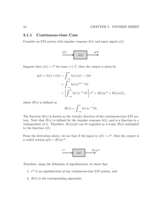
![3.1. EIGENFUNCTIONS OF AN LTI SYSTEM 45
If we specialize to the subclass of periodic complex exponentials of the ejωt
, ω ∈ R
by setting s = jω, then
H(s)|s=jω = H(jω) =
∞
−∞
h(τ)e−jωτ
dτ.
H(jω) is called the frequency response of the system.
3.1.2 Discrete-time Case
Next, we consider the discrete-time case:
Suppose that the impulse response is given by h[n] and the input is x[n] = zn
, then
the output y[n] is
y[n] = h[n] ∗ x[n] =
∞
k=−∞
h[k]x[n − k]
=
∞
k=−∞
h[k]zn−k
= zn
∞
k=−∞
h[k]z−k
= H(z)zn
,
where we defined
H(z) =
∞
k=−∞
h[k]z−k
,
and H(z) is known as the transfer function of the discrete-time LTI system.
Similar to the continuous-time case, this result indicates that
1. zn
is an eigenfunction of a discrete-time LTI system, and
2. H(z) is the corresponding eigenvalue.](https://image.slidesharecdn.com/note0-160519103024/85/Note-0-45-320.jpg)
![46 CHAPTER 3. FOURIER SERIES
Considering the subclass of periodic complex exponentials e−j(2π/N)n
by setting z =
ej2π/N
, we have
H(z)|z=ejΩ = H(ejΩ
) =
∞
k=−∞
h[k]e−jΩk
,
where Ω = 2π
N
, and H(ejΩ
) is called the frequency response of the system.
3.1.3 Summary
In summary, we have the following observations:
That is, est
is an eigenfunction of a CT system, whereas zn
is an eigenfunction of a
DT system. The corresponding eigenvalues are H(s) and H(z).
If we substitute s = jω and z = ejΩ
respectively, then the eigenfunctions become ejωt
and ejΩn
; the eigenvalues become H(jω) and H(ejΩ
).
3.1.4 Why is eigenfunction important?
The answer to this question is related to the second objective in the beginning. Let
us consider a signal x(t):
x(t) = a1es1t
+ a2es2t
+ a3es3t
.
According the eigenfunction analysis, the output of each complex exponential is
es1t
−→ H(s1)es1t
es2t
−→ H(s2)es2t
es3t
−→ H(s3)es3t
.](https://image.slidesharecdn.com/note0-160519103024/85/Note-0-46-320.jpg)
![3.2. FOURIER SERIES REPRESENTATION 47
Therefore, the output is
y(t) = a1H(s1)es1t
+ a2H(s2)es2t
+ a3H(s3)es3t
.
The result implies that if the input is a linear combination of complex exponentials,
the output of an LTI system is also a linear combination of complex exponentials.
More generally, if x(t) is an infinite sum of complex exponentials,
x(t) =
∞
k=−∞
akeskt
,
then the output is again a sum of complex exponentials:
y(t) =
∞
k=−∞
akH(sk)eskt
.
Similarly for discrete-time signals, if
x[n] =
∞
k=−∞
akzn
k ,
then
x[n] =
∞
k=−∞
akH(zk)zn
k .
This is an important observation, because as long as we can express a signal x(t) as
a linear combination of eigenfunctions, then the output y(t) can be easily determined
by looking at the transfer function (which is fixed for an LTI system!). Now, the
question is : How do we express a signal x(t) as a linear combination of complex
exponentials?
3.2 Fourier Series Representation
Existence of Fourier Series
In general, not every signal x(t) can be decomposed as a linear combination of complex
exponentials. However, such decomposition is still possible for an extremely large class
of signals. We want to study one class of signals that allows the decomposition. They
are the periodic signals
x(t + T) = x(t)](https://image.slidesharecdn.com/note0-160519103024/85/Note-0-47-320.jpg)
![3.2. FOURIER SERIES REPRESENTATION 49
Proof. Let us consider the signal
x(t) =
∞
k=−∞
akejkω0t
.
If we multiply on both sides e−jnω0t
, then we have
x(t)e−jnω0t
=
∞
k=−∞
akejkω0t
e−jnω0t
=
∞
k=−∞
akej(k−n)ω0t
.
Integrating both sides from 0 to T yields
T
0
x(t)e−jnω0t
dt =
T
0
∞
k=−∞
akej(k−n)ω0t
dt
=
∞
k=−∞
ak
T
0
ej(k−n)ω0t
dt .
The term
T
0
ej(k−n)ω0t
dt can be evaluated as (You should check this!)
1
T
T
0
ej(k−n)ω0t
dt =
1 if k = n
0 otherwise
(3.1)
This result is known as the orthogonality of the complex exponentials.
Using Eq. (3.1), we have
T
0
x(t)e−jnω0t
dt = Tan,
which is equivalent to
an =
1
T
T
0
x(t)e−jnω0t
dt.
Example 1. Sinusoids
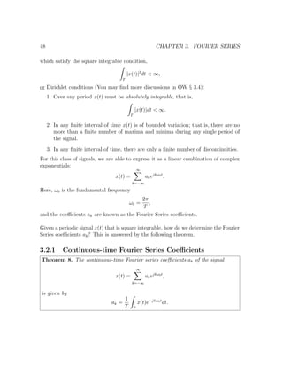
Consider the signal x(t) = 1+1
2
cos 2πt+sin 3πt. The period of x(t) is T = 2 [Why?] so
the fundamental frequency is ω0 = 2π
T
= π. Recall Euler’s formula ejθ
= cos θ+j sin θ,
we have
x(t) = 1 +
1
4
ej2πt
+ e−j2πt
+
1
2j
ej3πt
− e−j3πt
.](https://image.slidesharecdn.com/note0-160519103024/85/Note-0-49-320.jpg)
![50 CHAPTER 3. FOURIER SERIES
Therefore, the Fourier series coefficients are (just “read off” from this equation!):
a0 = 1, a1 = a−1 = 0, a2 = a−2 =
1
4
, a3 =
1
2j
, a−3 = −
1
2j
,
and ak = 0 otherwise.
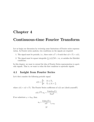
Example 2. Periodic Rectangular Wave
Let us determine the Fourier series coefficients of the following signal
x(t) =
1 |t| < T1,
0 T1 < |t| < T
2
.
The Fourier series coefficients are (k = 0):
ak =
1
T
T/2
−T/2
x(t)e−jkω0t
dt =
1
T
T1
−T1
e−jkω0t
dt
=
−1
jkω0T
e−jkω0t T1
−T1
=
2
kω0T
ejkω0T1
− e−jkω0T1
2j
=
2 sin(kω0T1)
kω0T
.
If k = 0, then
a0 =
1
T
T1
−T1
dt =
2T1
T
.
Example 3. Periodic Impulse Train
Consider the signal x(t) = ∞
k=−∞ δ(t − kT). The fundamental period of x(t) is T
[Why?]. The F.S. coefficients are
ak =
1
T
T/2
−T/2
δ(t)dt =
1
T
,
for any k.](https://image.slidesharecdn.com/note0-160519103024/85/Note-0-50-320.jpg)
![3.2. FOURIER SERIES REPRESENTATION 51
3.2.2 Discrete-time Fourier Series coefficients
To construct the discrete-time Fourier series representation, we consider periodic
discrete-time signal with period N
x[n] = x[n + N],
and assume that x[n] is square-summable, i.e., ∞
n=−∞ |x[n]|2
< ∞, or x[n] satisfies
the Dirichlet conditions. In this case, we have
Theorem 9. The discrete-time Fourier series coefficients ak of the signal
x[n] =
∞
k=−∞
akejkΩ0n
,
is given by
ak =
1
N
n= N
x[n]e−jkΩ0n
.
Here, n= N means summing the signal within a period N. Since a periodic discrete-
time signals repeats every N samples, it does not matter which sample to be picked
first.
Example.
Let us consider the following signal shown below. We want to determine the discrete-
time F.S. coefficient.](https://image.slidesharecdn.com/note0-160519103024/85/Note-0-51-320.jpg)
![52 CHAPTER 3. FOURIER SERIES
For k = 0, ±N, ±2N, . . ., we have
ak =
1
N
n= N
e−jkΩ0n
=
1
N
N1
n=−N1
e−jkΩ0n
=
1
N
2N1
m=0
e−jkΩ0(m−N1)
, (m = n + N0)
=
1
N
ejkΩ0N1
2N1
m=0
e−jkΩ0m
.
Since
2N1
m=0
e−jkΩ0m
=
1 − e−jkΩ0(2N1+1)
1 − e−jkΩ0
,
it follows that
ak =
1
N
ejkΩ0N1
1 − e−jkΩ0(2N1+1)
1 − e−jkΩ0
, (Ω0 = 2π/N)
=
1
N
e−jk(2π/2N)
[ejk2π(N1+1/2)/N
− e−jk2π(N1+1/2)/N
]
e−jk(2π/2N)[ejk(2π/2N) − e−jk(2π/2N)]
=
1
N
sin[2πk(N1 + 1/2)/N]
sin(πk
N
)
.
For k = 0, ±N, ±2N, . . ., we have
ak =
2N1 + 1
N
.
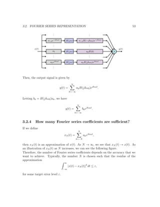
3.2.3 How do we use Fourier series representation?
Fourier series representation says that any periodic square integrable signals (or sig-
nals that satisfy Dirichlet conditions) can be expressed as a linear combination of
complex exponentials. Since complex exponentials are eigenfunctions to LTI sys-
tems, the output signal must be a linear combination of complex exponentials.
That is, for any signal x(t) we represent it as
x(t) =
∞
k=−∞
akejkω0t
.](https://image.slidesharecdn.com/note0-160519103024/85/Note-0-52-320.jpg)
![54 CHAPTER 3. FOURIER SERIES
3.3 Properties of Fourier Series Coefficients
There are a number of Fourier series properties that we encourage you to read the
text. The following is a quick summary of these properties.
1. Linearity: If x1(t) ←→ ak and x2(t) ←→ bk, then
Ax1(t) + Bx2(t) ←→ Aak + Bbk.
For DT case, we have if x1[n] ←→ ak and x2[n] ←→ bk, then
Ax1[n] + Bx2[n] ←→ Aak + Bbk.
2. Time Shift:
x(t − t0) ←→ ake−jkω0t0
x[n − n0] ←→ ake−jkΩ0n0
To show the time shifting property, let us consider the F.S. coefficient bk of the
signal y(t) = x(t − t0).
bk =
1
T T
x(t − t0)e−jω0t
dt.](https://image.slidesharecdn.com/note0-160519103024/85/Note-0-54-320.jpg)
![3.3. PROPERTIES OF FOURIER SERIES COEFFICIENTS 55
Letting τ = t − t0 in the integral, we obtain
1
T T
x(τ)e−jkω0(τ+t0)
dτ = e−jkω0t0
1
T T
x(τ)e−jkω0τ
dτ
where x(t) ←→ ak. Therefore,
x(t − t0) ←→ ake−jkω0t0
.
3. Time Reversal:
x(−t) ←→ a−k
x[−n] ←→ a−k
The proof is simple. Consider a signal y(t) = x(−t). The F.S. representation
of x(−t) is
x(−t) =
∞
k=−∞
ake−jk2πt/T
.
Letting k = −m, we have
y(t) = x(−t) =
∞
m=−∞
a−mejm2πt/T
.
Thus, x(−t) ←→ a−k.
4. Conjugation:
x∗
(t) ←→ a∗
−k
x∗
[n] ←→ a∗
−k
5. Multiplication: If x(t) ←→ ak and y(t) ←→ bk, then
x(t)y(t) ←→
∞
l=−∞
akbk−l.
6. Parseval Equality:
1
T T
|x(t)|2
dt =
∞
k=−∞
|ak|2
1
N
n= N
|x[n]|2
=
k= N
|ak|2
You are required to read Table 3.1 and 3.2.](https://image.slidesharecdn.com/note0-160519103024/85/Note-0-55-320.jpg)

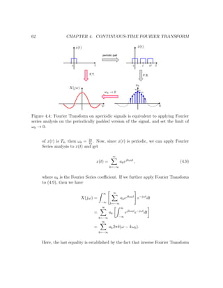
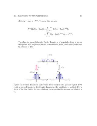
![66 CHAPTER 4. CONTINUOUS-TIME FOURIER TRANSFORM
Now, the second term is
lim
a→0
−j
ω
a2 + ω2
=
1
jω
.
The first term satisfies
lim
a→0
a
a2 + ω2
= 0, for ω = 0.
and
lim
a→0
a
a2 + ω2
= lim
a→0
1
a
= ∞, for ω = 0,
while ∞
−∞
a
a2 + ω2
dω = tan−1 ω
a
∞
−∞
= π, ∀ a ∈ R.
Therefore,
lim
a→0
a
a2 + ω2
= πδ(ω),
and so
U(jω) =
1
jω
+ πδ(ω).
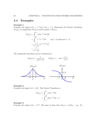
4.5 Properties of Fourier Transform
The properties of Fourier Transform is very similar to those of Fourier Series.
1. Linearity If x1(t) ←→ X1(jω) and x2(t) ←→ X2(jω), then
ax1(t) + bx2(t) ←→ aX1(jω) + bX2(jω).
2. Time Shifting
x(t − t0) ←→ e−jωt0
X(jω)
Physical interpretation of e−jωt0
:
e−jωt0
X(jω) = |X(jω)|ej X(jω)
e−jωt0
= |X(jω)|ej[ X(jω)−ωt0]
So e−jωt0
is contributing to phase shift of X(jω).](https://image.slidesharecdn.com/note0-160519103024/85/Note-0-66-320.jpg)
![68 CHAPTER 4. CONTINUOUS-TIME FOURIER TRANSFORM
8. Convolution Property
h(t) ∗ x(t) ←→ H(jω)X(jω)
Proof: Consider the convolution integral
y(t) =
∞
−∞
x(τ)h(t − τ)dτ
Taking Fourier Transform on both sides yields
Y (jω) = F
∞
−∞
x(τ)h(t − τ)dτ
=
∞
−∞
∞
−∞
x(τ)h(t − τ)dτ e−jωt
dt
=
∞
−∞
x(τ)
∞
−∞
h(t − τ)e−jωt
dt dτ
=
∞
−∞
x(τ) e−jωτ
H(jω) dτ
=
∞
−∞
x(τ)e−jωτ
dτH(jω)
= X(jω)H(jω)
9. Multiplication Property (you can derive this by yourself)
x(t)y(t) ←→
1
2π
X(jω) ∗ Y (jω)
Example.
Consider the signal x(t) = m(t) cos(ω0t), where m(t) is some bandlimited signal.
Suppose the Fourier Transform of m(t) is M(jω). Since
cos(ω0t) =
ejω0t
+ e−jω0t
2
←→ π[δ(ω − ω0) + δ(ω + ω0)],
by convolution property, the CTFT of x(t) is
m(t) cos(ω0t) ←→
1
2π
M(jω) ∗ π[δ(ω − ω0) + δ(ω + ω0)]
=
1
2
[M(j(ω − ω0)) + M(j(ω + ω0))] .](https://image.slidesharecdn.com/note0-160519103024/85/Note-0-68-320.jpg)
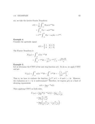
![74 CHAPTER 5. DISCRETE-TIME FOURIER TRANSFORM
By defining
X (jω) =
∞
−∞
x (t) ejωt
dt, (5.1)
which is known as the continuous-time Fourier Transform, we showed
ak =
1
T
X (jkω0) .
• Step 3: Setting T → ∞, we showed ˜x (t) → x (t) and
x (t) =
1
2π
∞
−∞
X (jω) ejωt
dt (5.2)
5.2 Deriving Discrete-time Fourier Transform
Now, let’s apply the same concept to discrete-time signals. In deriving the discrete-
time Fourier Transform, we also have three key steps.
• Step 1: Consider an aperiodic discrete-time signal x[n]. We pad x[n] to con-
struct a periodic signal ˜x[n].
• Step 2: Since ˜x[n] is periodic, by discrete-time Fourier Series we have
˜x[n] =
k= N
akejkω0n
, (5.3)
where ak can be computed as
ak =
1
N
n= N
˜x [n] ejkω0n
.](https://image.slidesharecdn.com/note0-160519103024/85/Note-0-74-320.jpg)
![5.2. DERIVING DISCRETE-TIME FOURIER TRANSFORM 75
Here, the frequency is
ω0 =
2π
N
.
Now, note that ˜x[n] is a periodic signal with period N, and the non-zero entries
of ˜x[n] in a period are the same as the non-zero entries of x[n]. Therefore, it
holds that
ak =
1
N
n= N
˜x [n] ejkω0n
=
1
N
∞
n=−∞
x [n] ejkω0n
.
If we define
X(ejω
) =
∞
n=−∞
x[n]e−jωn
, (5.4)
then
ak =
1
N
∞
n=−∞
x[n]ejkω0n
=
1
N
X(ejkω0
). (5.5)
• Step 3: Putting Equation (5.5) into Equation (5.3), we have
˜x[n] =
k= N
akejkω0n
=
k= N
1
N
X(ejkω0
) ejkω0n
=
1
2π
k= N
X(ejkω0
)ejkω0n
ω0, ω0 =
2π
N
. (5.6)
As N → ∞, ω0 → 0 and ˜x[n] → x[n]. Also, from Equation (5.6) becomes
˜x[n] =
1
2π
k= N
X(ejkω0
)ejkω0n
ω0 −→
1
2π 2π
X(ejω
)ejωn
dω.
Therefore,
x[n] =
1
2π 2π
X(ejω
)ejωn
dω. (5.7)](https://image.slidesharecdn.com/note0-160519103024/85/Note-0-75-320.jpg)
![76 CHAPTER 5. DISCRETE-TIME FOURIER TRANSFORM
Figure 5.1: As N → ∞, ω0 → 0. So the area becomes infinitesimal small and sum
becomes integration.
5.3 Why is X(ejω
) periodic ?
It is interesting to note that the continuous-time Fourier Transform X(jω) is aperiodic
in general, but the discrete-time Fourier Transform X(ejω
) is always periodic. To see
this, let us consider the discrete-time Fourier Transform (we want to check whether
X(ejω
) = X(ej(ω+2π)
)!):
X(ej(ω+2π)
) =
∞
n=−∞
x[n]e−j(ω+2π)n
=
∞
n=−∞
x[n]e−jωn
(e−j2π
)n
= X(ejω
),
because (e−j2π
)n
= 1n
= 1, for any integer n. Therefore, X(ejω
) is periodic with
period 2π.
Now, let us consider the continuous-time Fourier Transform (we want to check whether
X(jω) = X(j(ω + 2π))!):
X(j(ω + 2π)) =
∞
−∞
x(t)e−j(ω+2π)t
dt =
∞
−∞
x(t)e−jωt
(e−j2π
)t
dt.
Here, t ∈ R and is running from −∞ to ∞. Pay attention that e−j2πt
= 1 unless t is
an integer (which different from the discrete-time case where n is always an integer!).
Therefore,
∞
−∞
x(t)e−jωt
e−j2πt
dt =
∞
−∞
x(t)e−jωt
dt,](https://image.slidesharecdn.com/note0-160519103024/85/Note-0-76-320.jpg)
![5.4. PROPERTIES OF DISCRETE-TIME FOURIER TRANSFORM 77
(a) (ej2π
)n
= 1 for all n, because n is integer. (b) (ej2π
)t
= 1 unless t is an integer.
and consequently,
X(j(ω + 2π)) = X(jω).
5.4 Properties of Discrete-time Fourier Transform
Discrete-time Fourier Transform:
X(ejω
) =
∞
n=−∞
x[n]e−jωn
Discrete-time Inverse Fourier Transform:
x[n] =
1
2π 2π
X(ejω
)ejωn
dω
1. Periodicity:
X(ej(ω+2π)
) = X(ejω
)
2. Linearity:
ax1[n] + bx2[n] ←→ aX1(ejω
) + bX2(ejω
)
3. Time Shift:
x[n − n0] ←→ e−jωn0
X(ejω
)
4. Phase Shift:
ejω0n
x[n] ←→ X(ej(ω−ω0)
)](https://image.slidesharecdn.com/note0-160519103024/85/Note-0-77-320.jpg)
![78 CHAPTER 5. DISCRETE-TIME FOURIER TRANSFORM
5. Conjugacy:
x∗
[n] ←→ X∗
(e−jω
)
6. Time Reversal
x[−n] ←→ X(e−jω
)
7. Differentiation
nx[n] ←→ j
dX(ejω
)
dω
8. Parseval Equality
∞
n=−∞
|x[n]|2
=
1
2π 2π
|X(ejω
)|2
dω
9. Convolution
y[n] = x[n] ∗ h[n] ←→ Y (ejω
) = X(ejω
)H(ejω
)
10. Multiplication
y[n] = x1[n]x2[n] ←→ Y (ejω
) =
1
2π 2π
X1(ejω
)X2(ej(ω−θ)
)dθ
5.5 Examples
Example 1.
Consider x[n] = δ[n] + δ[n − 1] + δ[n + 1]. Then
X(ejω
) =
∞
n=−∞
x[n]e−jωn
=
∞
n=−∞
(δ[n] + δ[n − 1] + δ[n + 1])e−jωn
=
∞
n=−∞
δ[n]e−jωn
+
∞
n=−∞
δ[n − 1]e−jωn
+
∞
n=−∞
δ[n + 1]e−jωn
= 1 + e−jω
+ ejω
= 1 + 2 cos ω.](https://image.slidesharecdn.com/note0-160519103024/85/Note-0-78-320.jpg)
![5.5. EXAMPLES 79
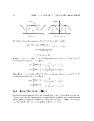
Figure 5.2: Magnitude plot of |X(ejω
)| in Example 1.
To sketch the magnitude |X(ejω
)|, we note that |X(ejω
)| = |1 + 2 cos ω|.
Example 2.
Consider x[n] = δ[n] + 2δ[n − 1] + 4δ[n − 2]. The discrete-time Fourier Transform is
X(ejω
) = 1 + 2e−jω
+ 4e−j4ω
.
If the impulse response is h[n] = δ[n] + δ[n − 1], then
H(ejω
) = 1 + e−jω
.
Therefore, the output is
Y (ejω
) = H(ejω
)X(ejω
)
= 1 + e−jω
1 + 2e−jω
+ 4e−j2ω
= 1 + 3e−jω
+ 6e−j2ω
+ 4e−j3ω
.
Taking the inverse discrete-time Fourier Transform, we have
y[n] = δ[n] + 3δ[n − 1] + 6δ[n − 2] + 4δ[n − 3].
Example 3.
Consider x[n] = an
u[n], with |a| < 1. The discrete-time Fourier Transform is
X(ejω
) =
∞
n=0
an
e−jωn
=
∞
n=0
(ae−jω
)n
=
1
1 − ae−jω
.](https://image.slidesharecdn.com/note0-160519103024/85/Note-0-79-320.jpg)
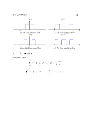
![84 CHAPTER 6. SAMPLING THEOREM
where T is the period of the impulse train. Multiplying x(t) with p(t) yields
xp(t) = x(t)p(t)
= x(t)
∞
n=−∞
δ(t − nT)
=
∞
n=−∞
x(t)δ(t − nT)
=
∞
n=−∞
x(nT)δ(t − nT).
Pictorially, xp(t) is a set of impulses bounded by the envelop x(t) as shown in Fig.
6.2.
Figure 6.2: An example of A/D conversion. The output signal xp(t) represents a set
of samples of the signal x(t).
We may regard xp(t) as the samples of x(t). Note that xp(t) is still a continuous-time
signal! (We can view xp(t) as a discrete-time signal if we define xp[n] = x(nT). But
this is not an important issue here.)
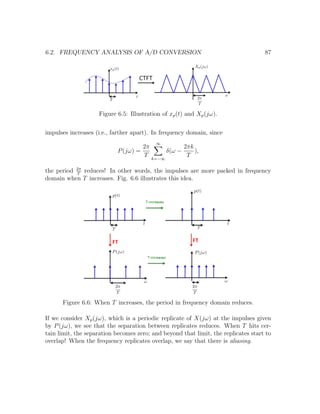
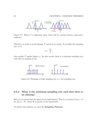
6.2 Frequency Analysis of A/D Conversion
Having an explanation of the A/D conversion in time domain, we now want to study
the A/D conversion in the frequency domain. (Why? We need it for the develop-
ment of Sampling Theorem!) So, how do the frequency responses X(jω), P(jω) and
Xp(jω) look like?](https://image.slidesharecdn.com/note0-160519103024/85/Note-0-84-320.jpg)
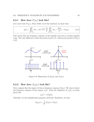
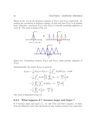
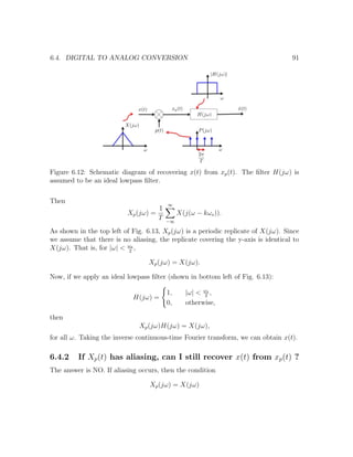

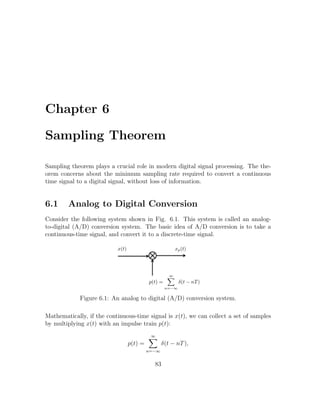
![Chapter 7
The z-Transform
The z-transform is a generalization of the discrete-time Fourier transform we learned
in Chapter 5. As we will see, z-transform allows us to study some system properties
that DTFT cannot do.
7.1 The z-Transform
Definition 21. The z-transform of a discrete-time signal x[n] is:
X(z) =
∞
n=−∞
x[n]z−n
. (7.1)
We denote the z-transform operation as
x[n] ←→ X(z).
In general, the number z in (7.1) is a complex number. Therefore, we may write z as
z = rejw
,
where r ∈ R and w ∈ R. When r = 1, (7.1) becomes
X(ejw
) =
∞
n=−∞
x[n]e−jwn
,
which is the discrete-time Fourier transform of x[n]. Therefore, DTFT is a special
case of the z-transform! Pictorially, we can view DTFT as the z-transform evaluated
on the unit circle:
95](https://image.slidesharecdn.com/note0-160519103024/85/Note-0-95-320.jpg)
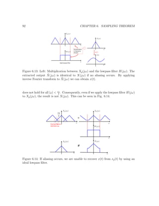
![96 CHAPTER 7. THE Z-TRANSFORM
Figure 7.1: Complex z-plane. The z-transform reduces to DTFT for values of z on
the unit circle.
When r = 1, the z-transform is equivalent to
X(rejw
) =
∞
−∞
x[n] rejw −n
=
∞
−∞
r−n
x[n] e−jwn
= F r−n
x[n] ,
which is the DTFT of the signal r−n
x[n]. However, from the development of DTFT
we know that DTFT does not always exist. It exists only when the signal is square
summable, or satisfies the Dirichlet conditions. Therefore, X(z) does not always
converge. It converges only for some values of r. This range of r is called the region
of convergence.
Definition 22. The Region of Convergence (ROC) of the z-transform is the set of
z such that X(z) converges, i.e.,
∞
n=−∞
|x[n]|r−n
< ∞.](https://image.slidesharecdn.com/note0-160519103024/85/Note-0-96-320.jpg)
![7.1. THE Z-TRANSFORM 97
Example 1. Consider the signal x[n] = an
u[n], with 0 < a < 1. The z-transform of
x[n] is
X(z) =
∞
−∞
an
u[n]z−n
=
∞
n=0
az−1 n
.
Therefore, X(z) converges if ∞
n=0 (az−1
)
n
< ∞. From geometric series, we know
that
∞
n=0
rz−1 n
=
1
1 − az−1
,
when |az−1
| < 1, or equivalently |z| > |a|. So,
X(z) =
1
1 − ax−1
,
with ROC being the set of z such that |z| > |a|.
Figure 7.2: Pole-zero plot and ROC of Example 1.](https://image.slidesharecdn.com/note0-160519103024/85/Note-0-97-320.jpg)
![98 CHAPTER 7. THE Z-TRANSFORM
Example 2. Consider the signal x[n] = −an
u[−n − 1] with 0 < a < 1. The
z-transform of x[n] is
X(z) = −
∞
n=−∞
an
u[−n − 1]z−n
= −
−1
n=−∞
an
z−n
= −
∞
n=1
a−n
zn
= 1 −
∞
n=0
a−1
z
n
.
Therefore, X(z) converges when |a−1
z| < 1, or equivalently |z| < |a|. In this case,
X(z) = 1 −
1
1 − a−1z
=
1
1 − az−1
,
with ROC being the set of z such that |z| < |a|. Note that the z-transform is the
same as that of Example 1. The only difference is the ROC. In fact, Example 2 is
just the left-sided version of Example 1!
Figure 7.3: Pole-zero plot and ROC of Example 2.](https://image.slidesharecdn.com/note0-160519103024/85/Note-0-98-320.jpg)
![7.1. THE Z-TRANSFORM 99
Example 3. Consider the signal
x[n] = 7
1
3
n
u[n] − 6
1
2
n
u[n].
The z-transform is
X(z) =
∞
n=−∞
7
1
3
n
− 6
1
2
n
u[n]z−n
= 7
∞
n=−∞
1
3
n
u[n]z−n
− 6
∞
n=−∞
1
2
n
u[n]z−n
= 7
1
1 − 1
3
z−1
− 6
1
1 − 1
2
z−1
=
1 − 3
2
z−1
1 − 1
3
z−1 1 − 1
2
z−1
.
For X(z) to converge, both sums in X(z) must converge. So we need both |z| > |1
3
|
and |z| > |1
2
|. Thus, the ROC is the set of z such that |z| > |1
2
|.
Figure 7.4: Pole-zero plot and ROC of Example 3.](https://image.slidesharecdn.com/note0-160519103024/85/Note-0-99-320.jpg)
![100 CHAPTER 7. THE Z-TRANSFORM
7.2 z-transform Pairs
7.2.1 A. Table 10.2
1. δ[n] ←→ 1, all z
2. δ[n − m] ←→ z−m
, all z except 0 when m > 0 and ∞ when m < 0.
3. u[n] ←→ 1
1−z−1 , |z| > 1
4. an
u[n] ←→ 1
1−az−1 , |z| > a
5. −an
u[−n − 1] ←→ 1
1−az−1 , |z| < |a|.
Example 4. Let us show that δ[n] ←→ 1. To see this,
X(z) =
∞
n=−∞
x[n]z−n
=
∞
n=−∞
δ[n]z−n
=
∞
n=−∞
δ[n] = 1.
Example 5. Let’s show that δ[n − m] ←→ z−m
:
X(z) =
∞
n=−∞
x[n]z−n
=
∞
n=−∞
δ[n − m]z−n
= z−m
∞
n=−∞
δ[n − m] = z−m
.
7.2.2 B. Table 10.1
1. ax1[n] + bx2[n] ←→ aX1(z) + bX2(z)
2. x[n − n0] ←→ X(z)z−n0
3. zn
0 x[n] ←→ X( z
z0
)
4. ejw0n
x[n] ←→ X(e−jw0
z)
5. x[−n] ←→ X(1
z
)](https://image.slidesharecdn.com/note0-160519103024/85/Note-0-100-320.jpg)
![7.2. Z-TRANSFORM PAIRS 101
6. x∗
[n] ←→ X∗
(z∗
)
7. x1[n] ∗ x2[n] ←→ X1(z)X2(z)
8. If y[n] =
x[n/L], n is multiples of L
0, otherwise,
then Y (z) = X(zL
).
Example 6. Consider the signal h[n] = δ[n] + δ[n − 1] + 2δ[n − 2]. The z-Transform
of h[n] is
H(z) = 1 + z−1
+ 2z−2
.
Example 7. Let prove that x[−n] ←→ X(z−1
). Letting y[n] = x[−n], we have
Y (z) =
∞
n=−∞
y[n]z−n
=
∞
n=−∞
x[−n]z−n
=
∞
m=−∞
x[m]zm
= X(1/z).
Example 8. Consider the signal x[n] = 1
3
sin π
4
n u[n]. To find the z-Transform,
we first note that
x[n] =
1
2j
1
3
ej π
4
n
u[n] −
1
2j
1
3
e−j π
4
n
u[n].
The z-Transform is
X(z) =
∞
n=−∞
x[n]z−n
=
∞
n=0
1
2j
1
3
ej π
4 z−1
n
−
∞
n=0
1
2j
1
3
e−j π
4 z−1
n
=
1
2j
1
1 − 1
3
ej π
4 z−1
−
1
2j
1
1 − 1
3
e−j π
4 z−1
=
1
3
√
2
z−1
(1 − 1
3
ej π
4 z−1)(1 − 1
3
e−j π
4 z−1)
.](https://image.slidesharecdn.com/note0-160519103024/85/Note-0-101-320.jpg)
![102 CHAPTER 7. THE Z-TRANSFORM
7.3 Properties of ROC
Property 1. The ROC is a ring or disk in the z-plane center at origin.
Property 2. DTFT of x[n] exists if and only if ROC includes the unit circle.
Proof. By definition, ROC is the set of z such that X(z) converges. DTFT is the z-
transform evaluated on the unit circle. Therefore, if ROC includes the unit circle, then
X(z) converges for any value of z on the unit circle. That is, DTFT converges.
Property 3. The ROC contains no poles.
Property 4. If x[n] is a finite impulse response (FIR), then the ROC is the entire
z-plane.
Property 5. If x[n] is a right-sided sequence, then ROC extends outward from the
outermost pole.
Property 6. If x[n] is a left-sided sequence, then ROC extends inward from the
innermost pole.
Proof. Let’s consider the right-sided case. Note that it is sufficient to show that if a
complex number z with magnitude |z| = r0 is inside the ROC, then any other complex
number z with magnitude |z | = r1 > r0 will also be in the ROC.
Now, suppose x[n] is a right-sided sequence. So, x[n] is zero prior to some values of
n, say N1. That is
x[n] = 0, n ≤ N1.
Consider a point z with |z| = r0, and r0 < 1. Then
X(z) =
∞
n=−∞
x[n]z−n
=
∞
n=N1
x[n]r−n
0 < ∞,](https://image.slidesharecdn.com/note0-160519103024/85/Note-0-102-320.jpg)
![7.3. PROPERTIES OF ROC 103
because r0 < 1 guarantees that the sum is finite.
Now, if there is another point z with |z | = r1 > r0, we may write r1 = ar0 for some
a > 1. Then the series
∞
n=N1
x[n]r−n
1 =
∞
n=N1
x[n]a−n
r−n
0
≤ aN1
∞
n=N1
x[n]r−n
0 < ∞.
So, z is also in the ROC.
Property 7. If X(z) is rational, i.e., X(z) = A(z)
B(z)
where A(z) and B(z) are poly-
nomials, and if x[n] is right-sided, then the ROC is the region outside the outermost
pole.
Proof. If X(z) is rational, then by (Appendix, A.57) of the textbook
X(z) =
A(z)
B(z)
=
n−1
k=0 akzk
r
k=1(1 − p−1
k z)σk
,
where pk is the k-th pole of the system. Using partial fraction, we have
X(z) =
r
i=1
σi
k=1
Cik
(1 − p−1
i z)k
.
Each of the term in the partial fraction has an ROC being the set of z such that
|z| > |pi| (because x[n] is right-sided). In order to have X(z) convergent, the ROC
must be the intersection of all individual ROCs. Therefore, the ROC is the region
outside the outermost pole.
For example, if
X(z) =
1
(1 − 1
3
z−1)(1 − 1
2
z−1)
,
then the ROC is the region |z| > 1
2
.](https://image.slidesharecdn.com/note0-160519103024/85/Note-0-103-320.jpg)
![104 CHAPTER 7. THE Z-TRANSFORM
7.4 System Properties using z-transform
7.4.1 Causality
Property 8. A discrete-time LTI system is causal if and only if ROC is the exterior
of a circle (including ∞).
Proof. A system is causal if and only if
h[n] = 0, n < 0.
Therefore, h[n] must be right-sided. Property 5 implies that ROC is outside a circle.
Also, by the definition that
H(z) =
∞
n=0
h[n]z−n
where there is no positive powers of z, H(z) converges also when z → ∞ (Of course,
|z| > 1 when z → ∞!).
7.4.2 Stablility
Property 9. A discrete-time LTI system is stable if and only if ROC of H(z)
includes the unit circle.
Proof. A system is stable if and only if h[n] is absolutely summable, if and only if
DTFT of h[n] exists. Consequently by Property 2, ROC of H(z) must include the
unit circle.
Property 10. A causal discrete-time LTI system is stable if and only if all of its
poles are inside the unit circle.
Proof. The proof follows from Property 8 and 9 directly.](https://image.slidesharecdn.com/note0-160519103024/85/Note-0-104-320.jpg)


![Script md a[1]](https://cdn.slidesharecdn.com/ss_thumbnails/script-mda1-101011070309-phpapp01-thumbnail.jpg?width=640&height=640&fit=bounds)