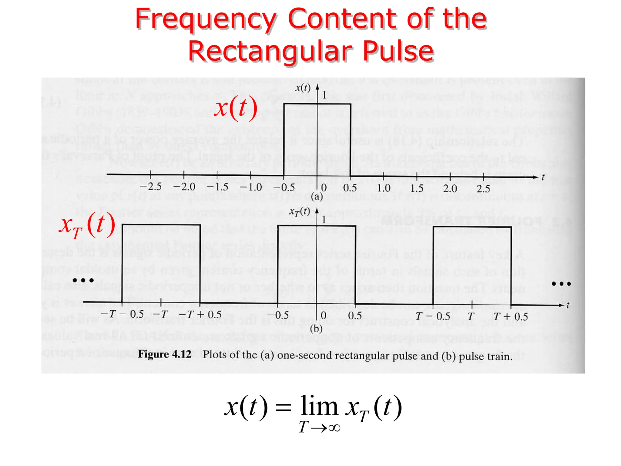
1. The document discusses Fourier analysis techniques for representing signals, including Fourier series and the Fourier transform. It uses the example of a rectangular pulse train to illustrate these concepts.
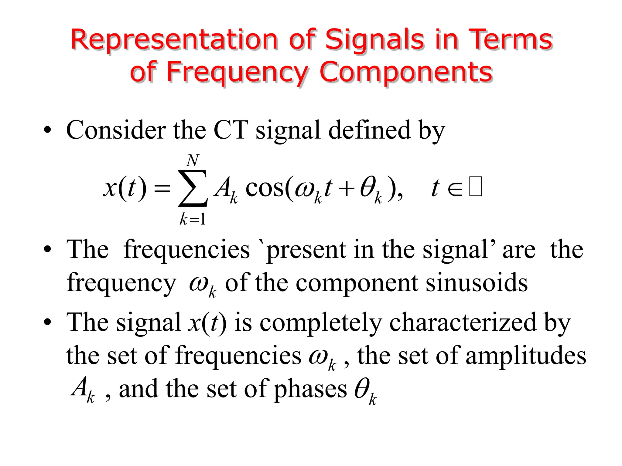
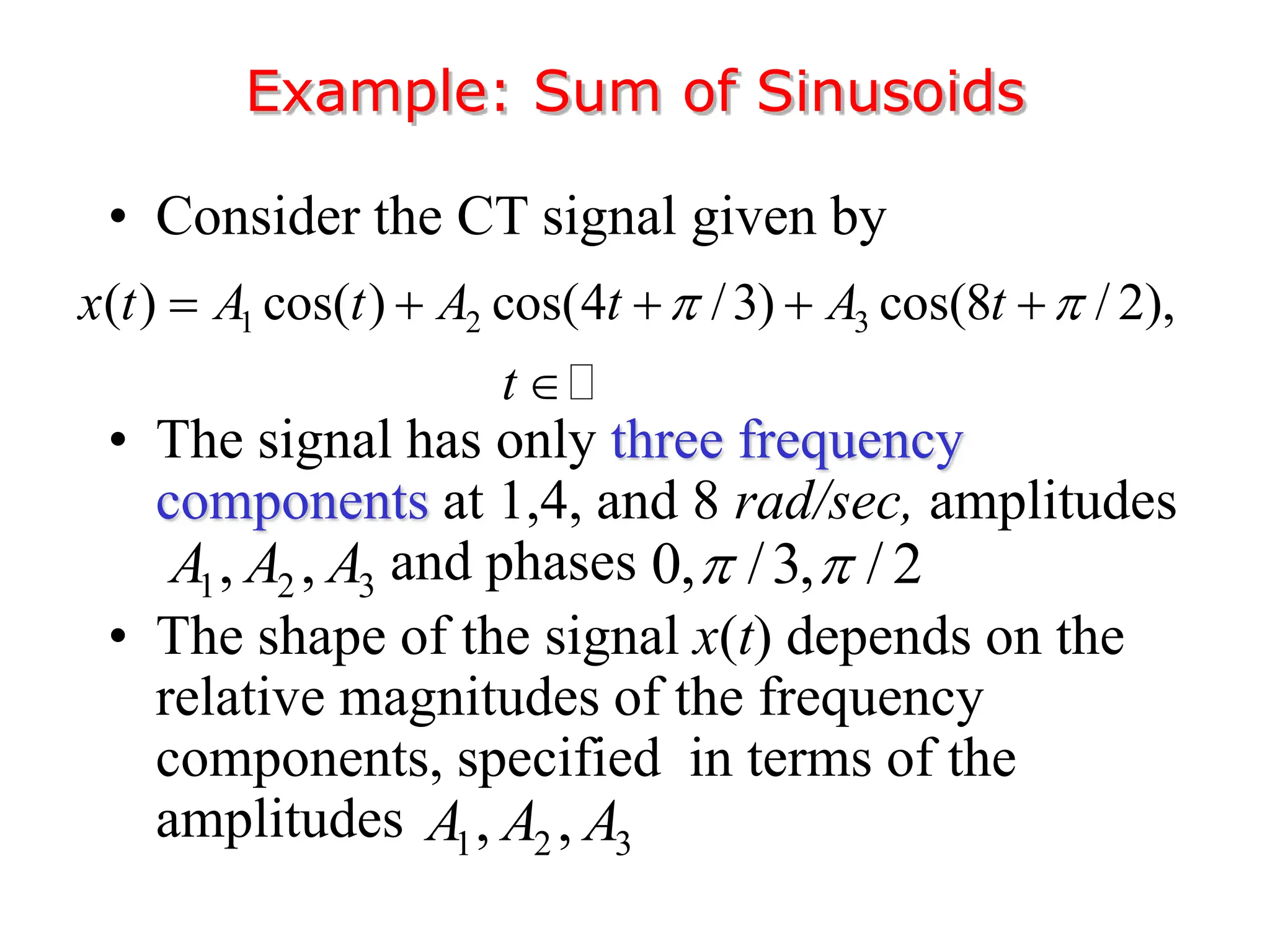
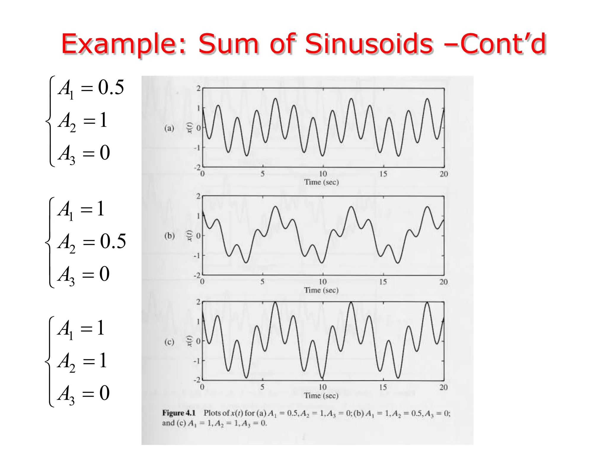
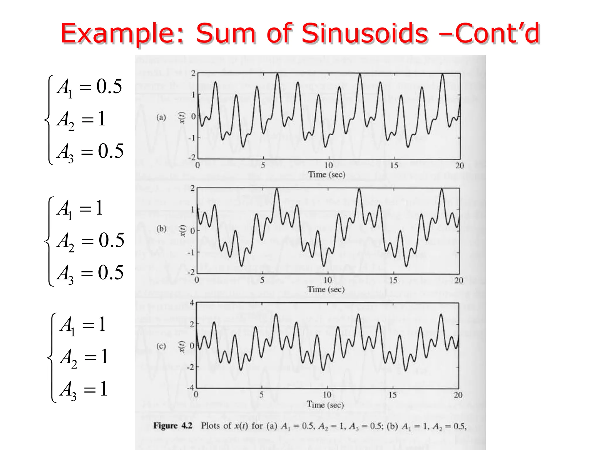
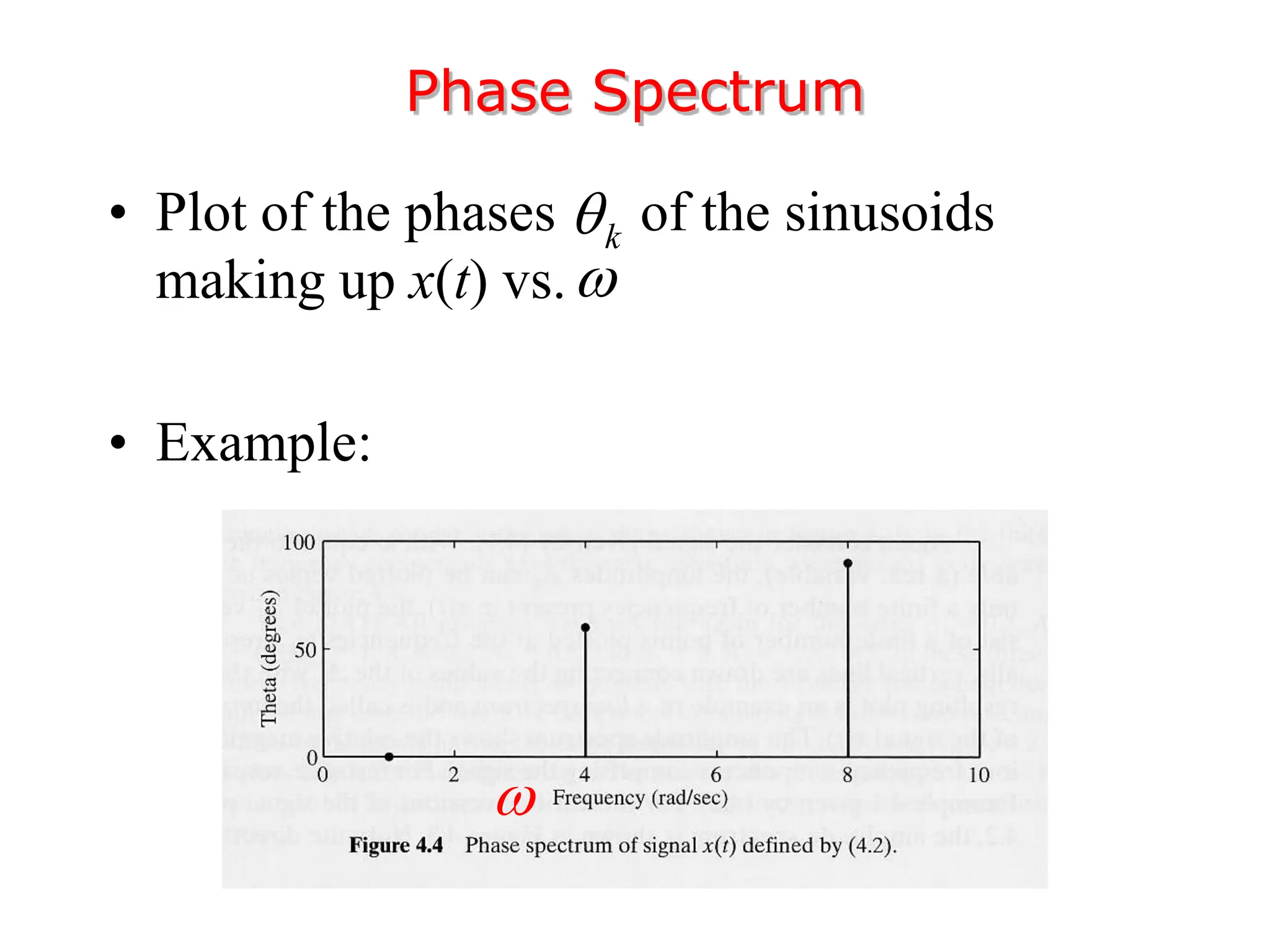
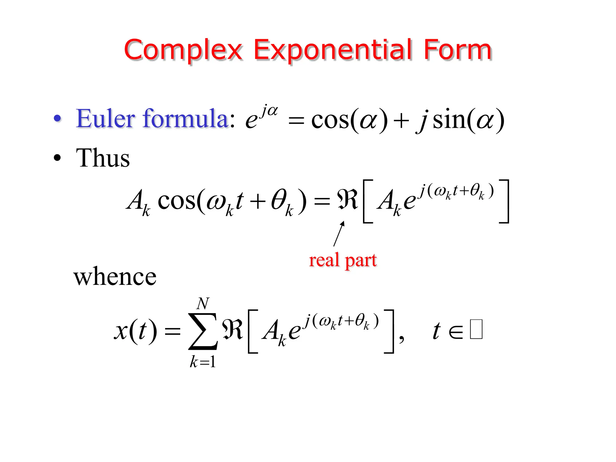
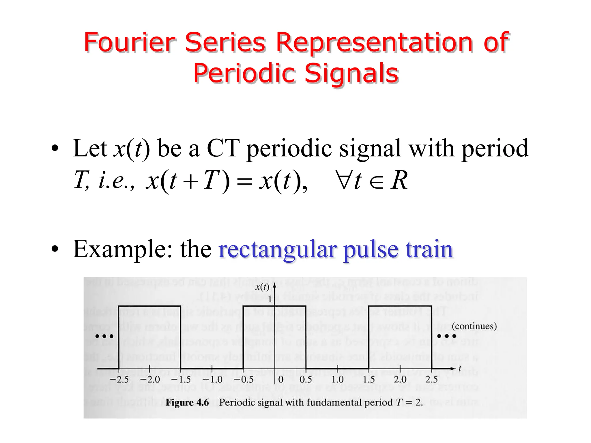
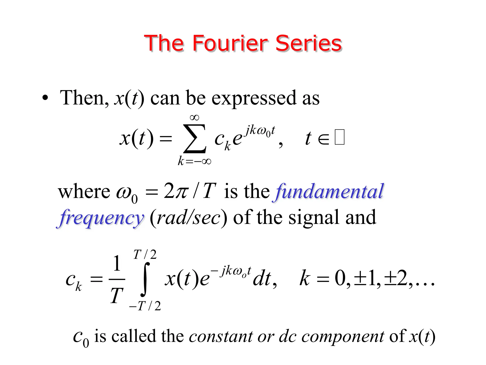
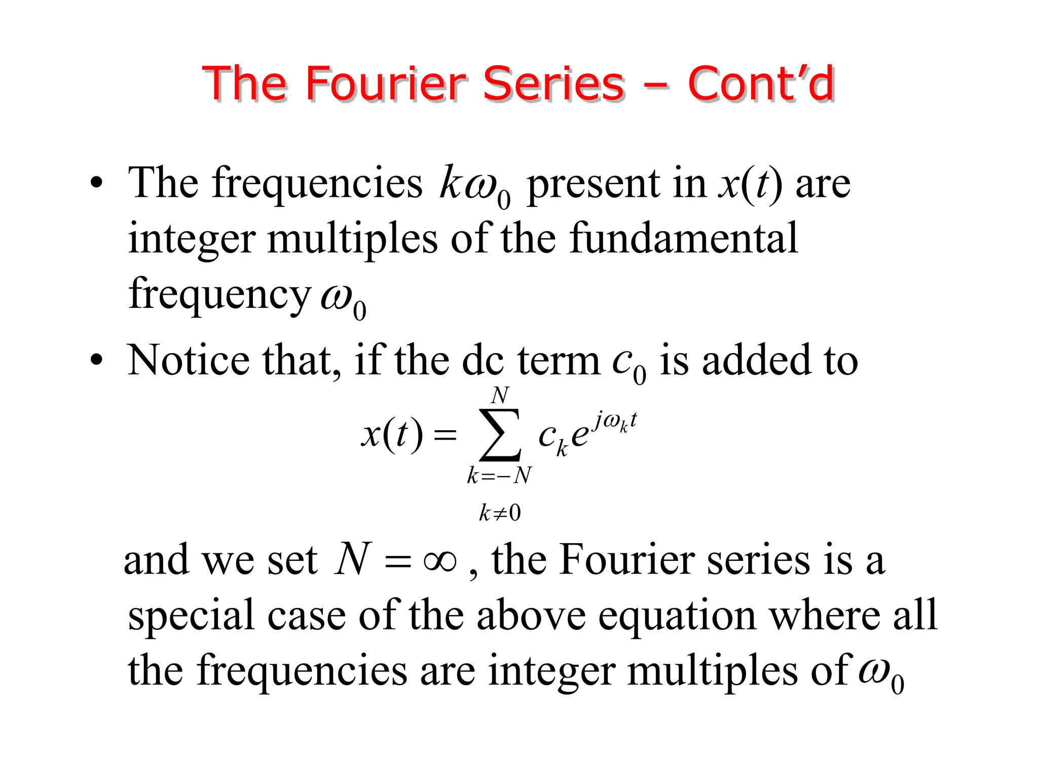
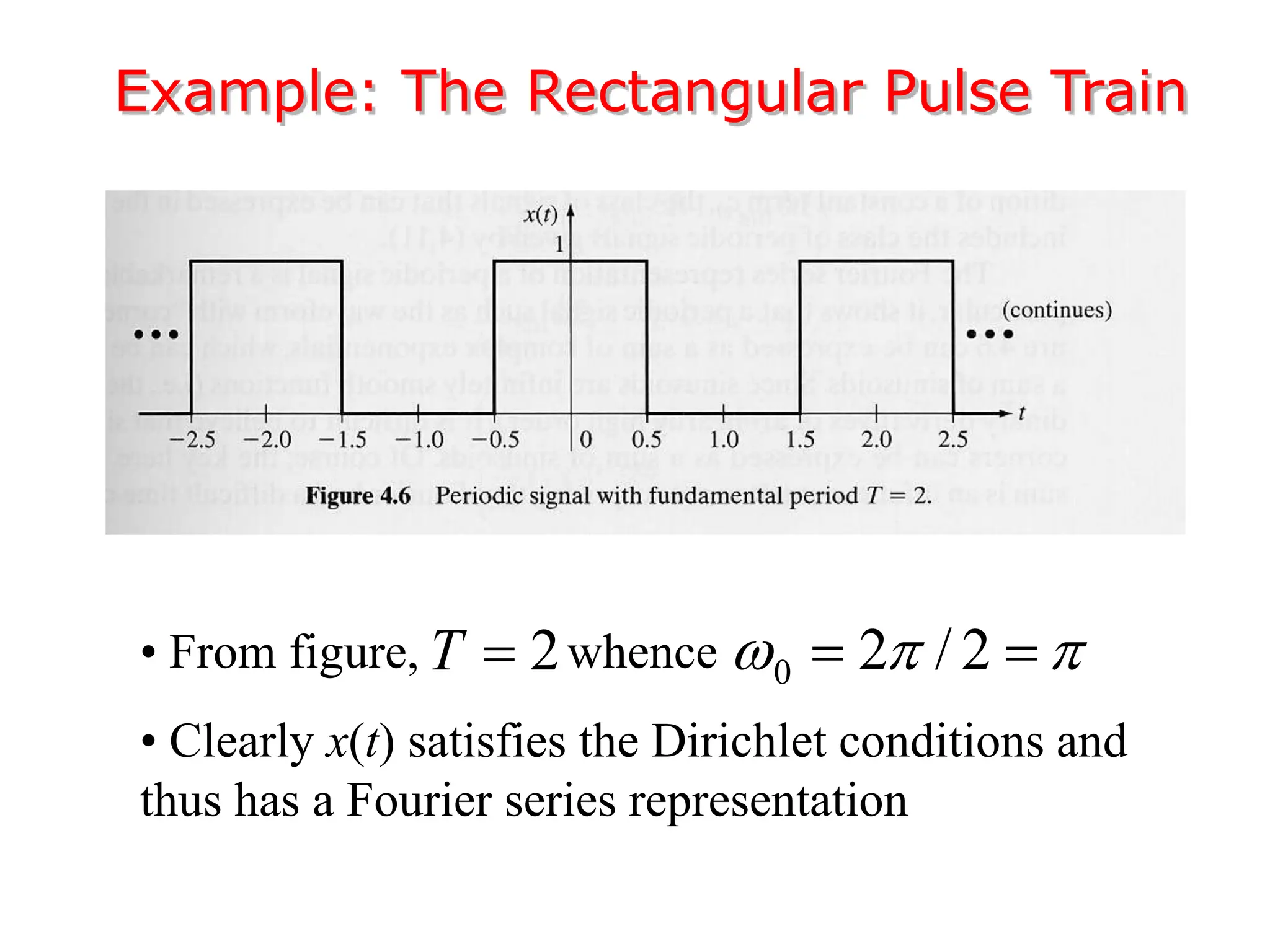
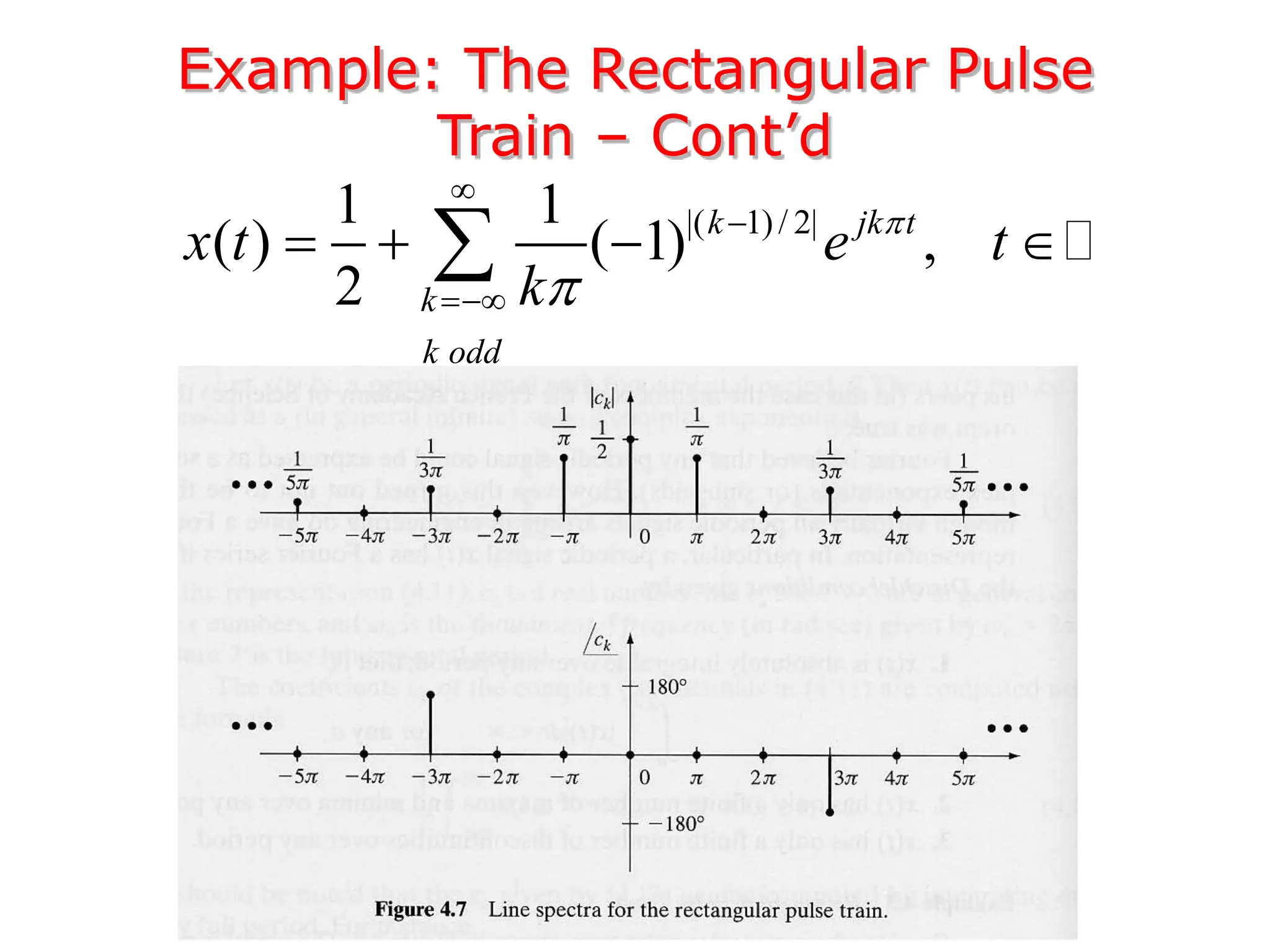
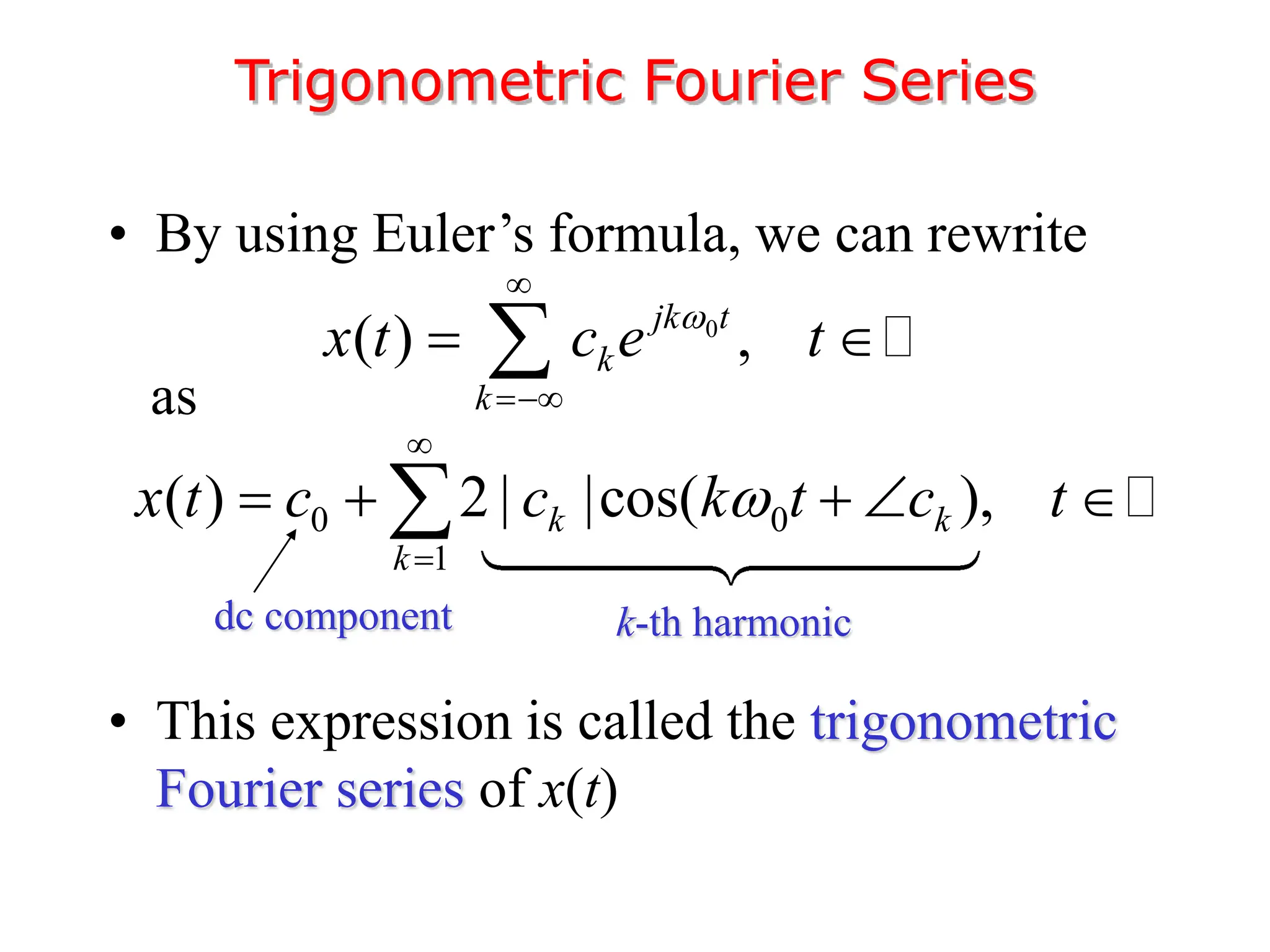
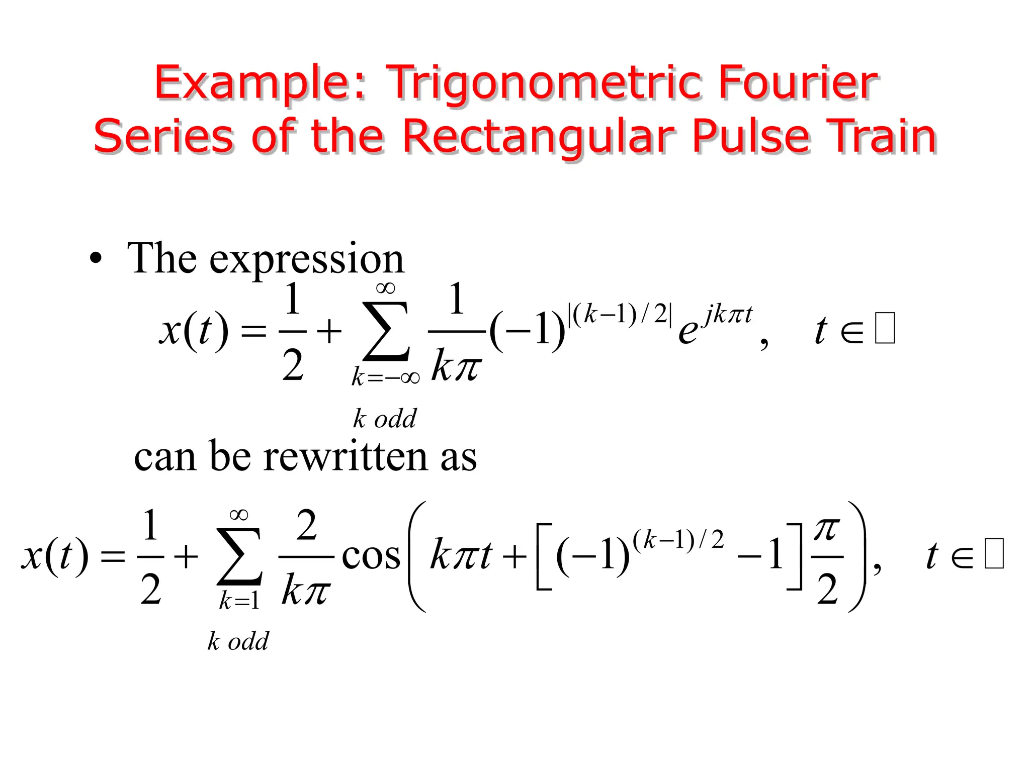
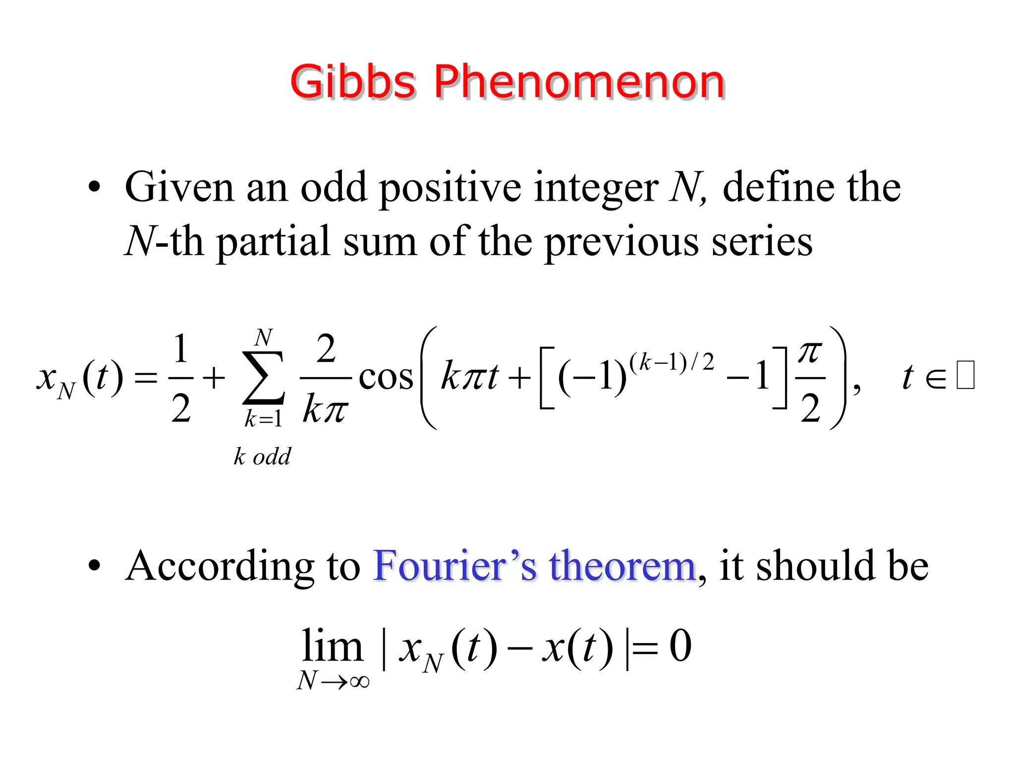
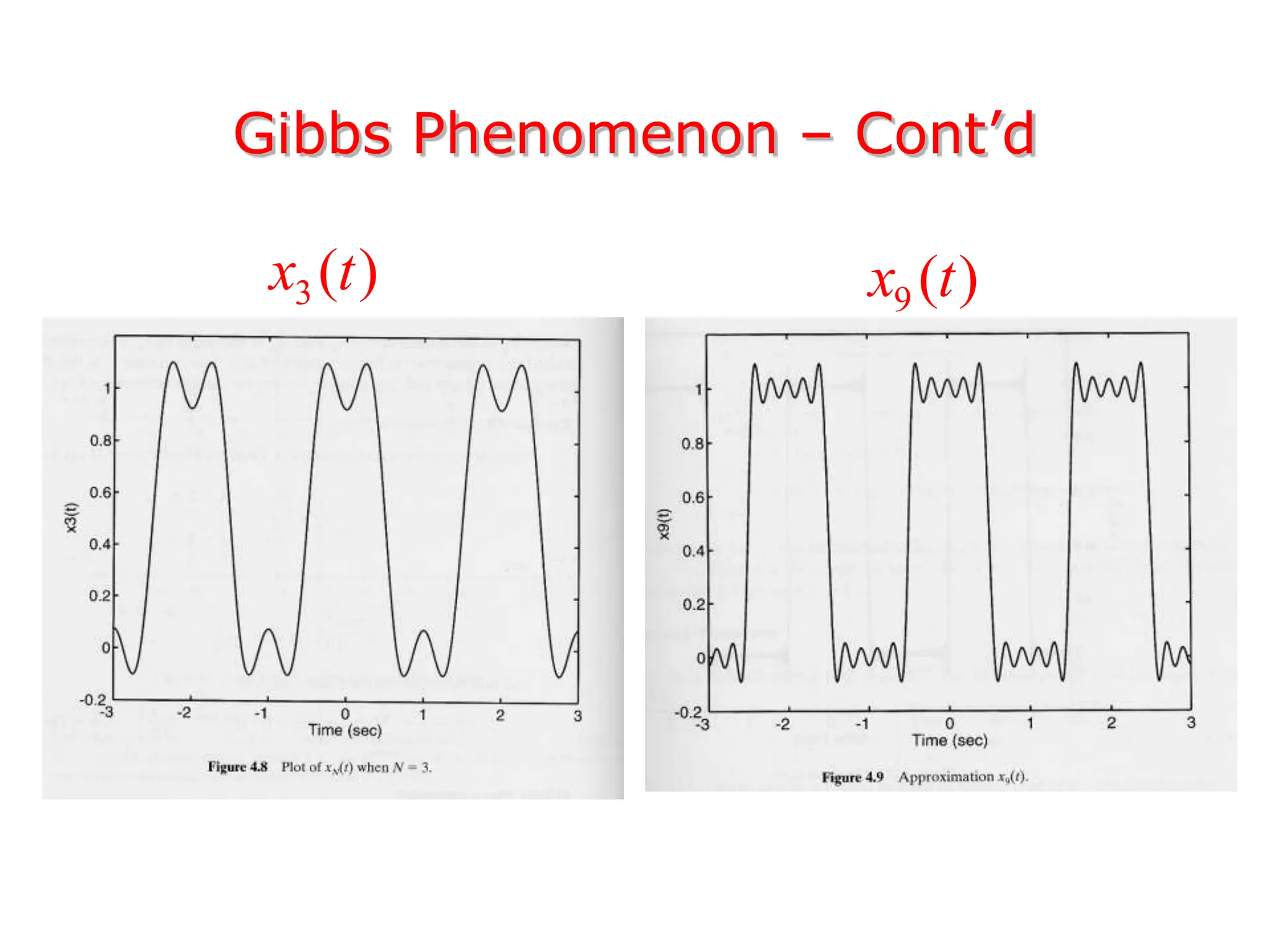
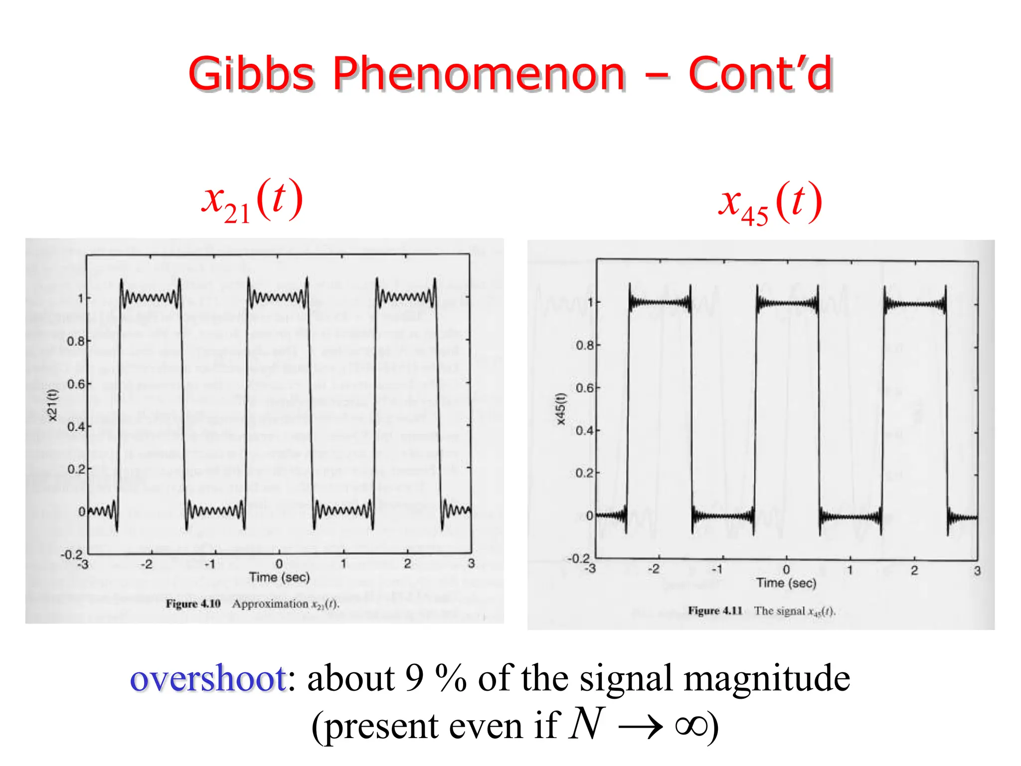
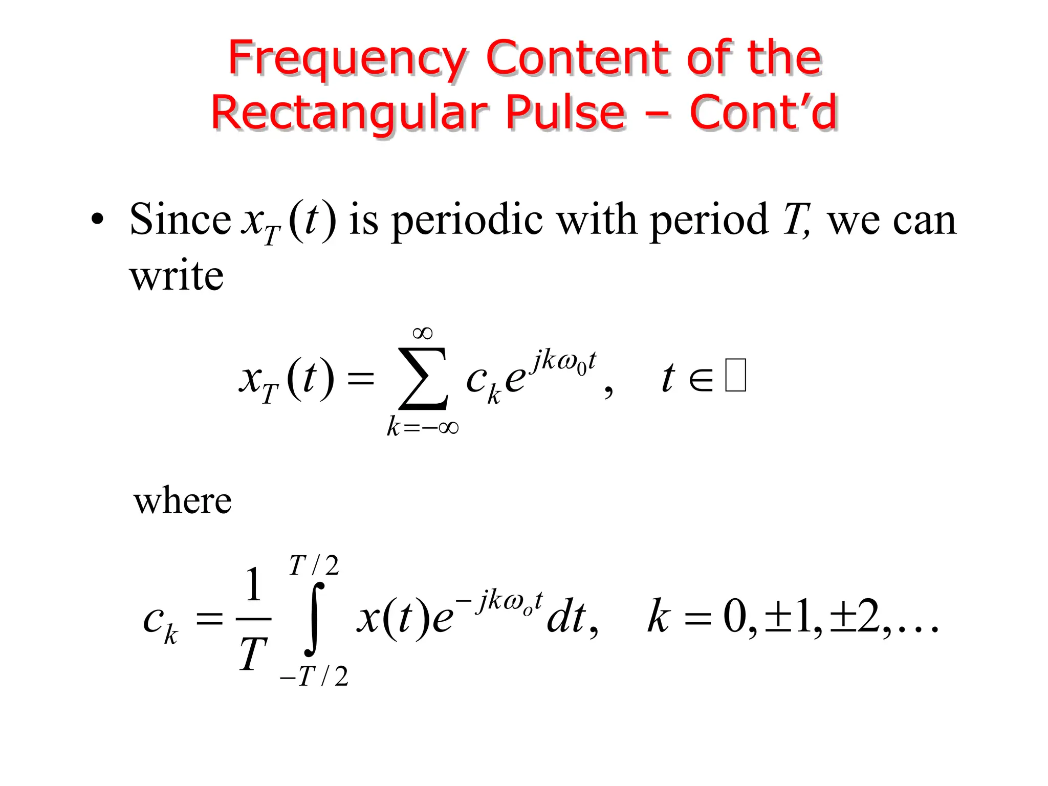
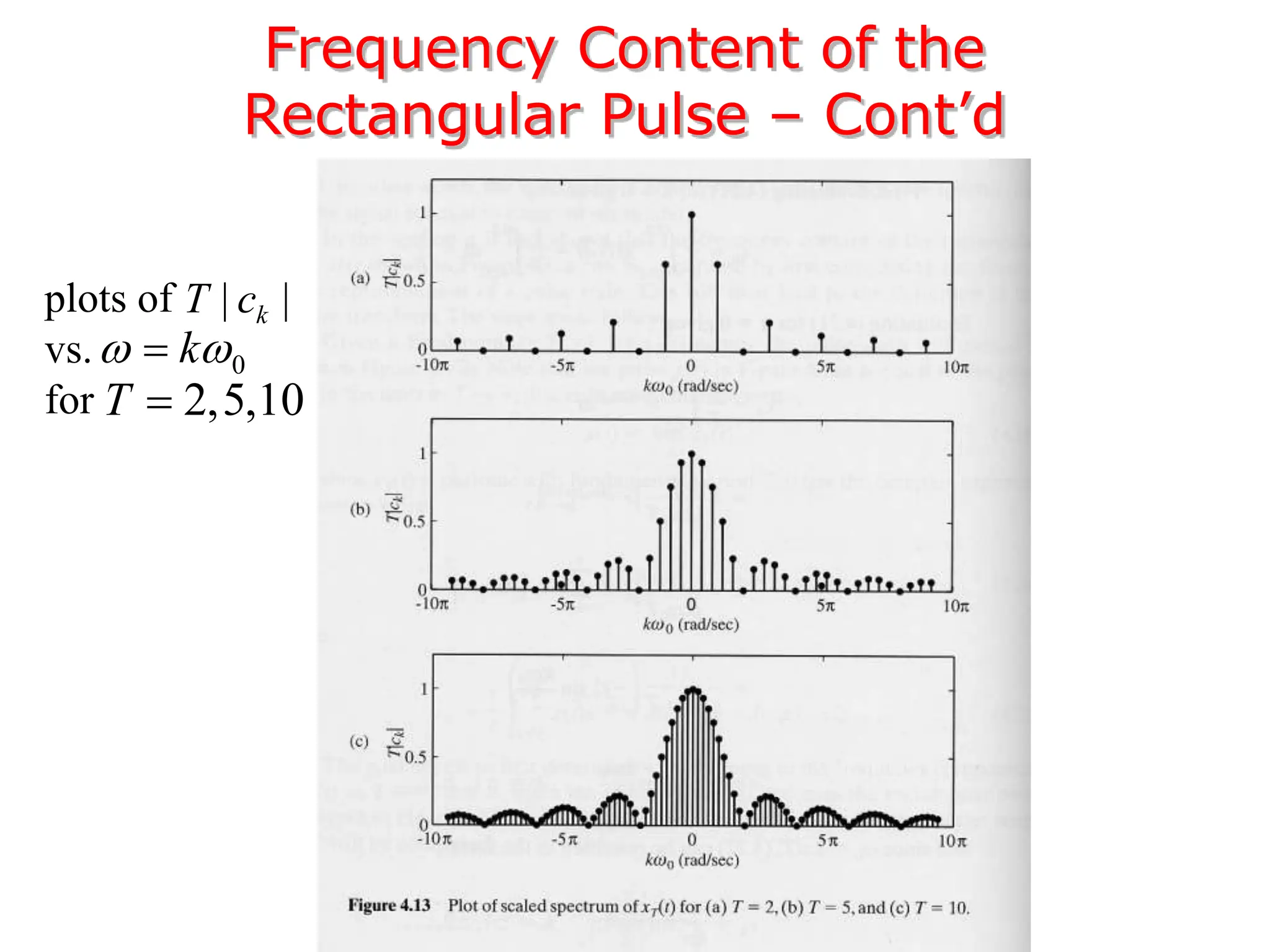
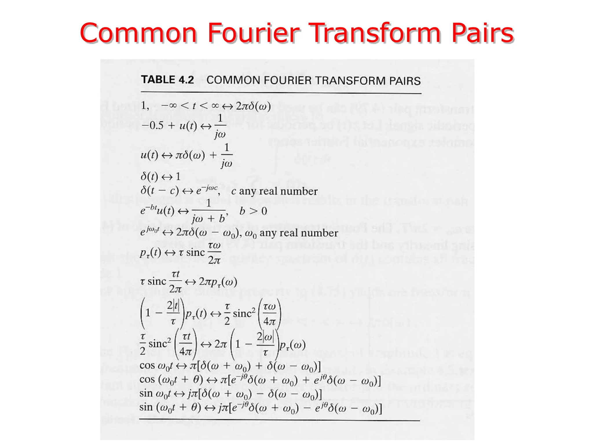
2. A periodic signal like a rectangular pulse train can be represented by a Fourier series as a sum of sinusoids with frequencies that are integer multiples of the fundamental frequency.
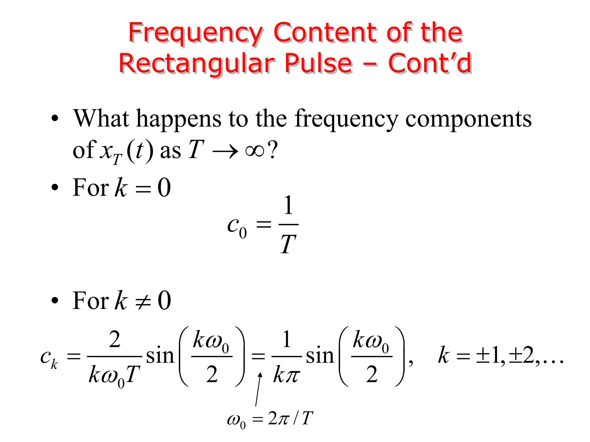
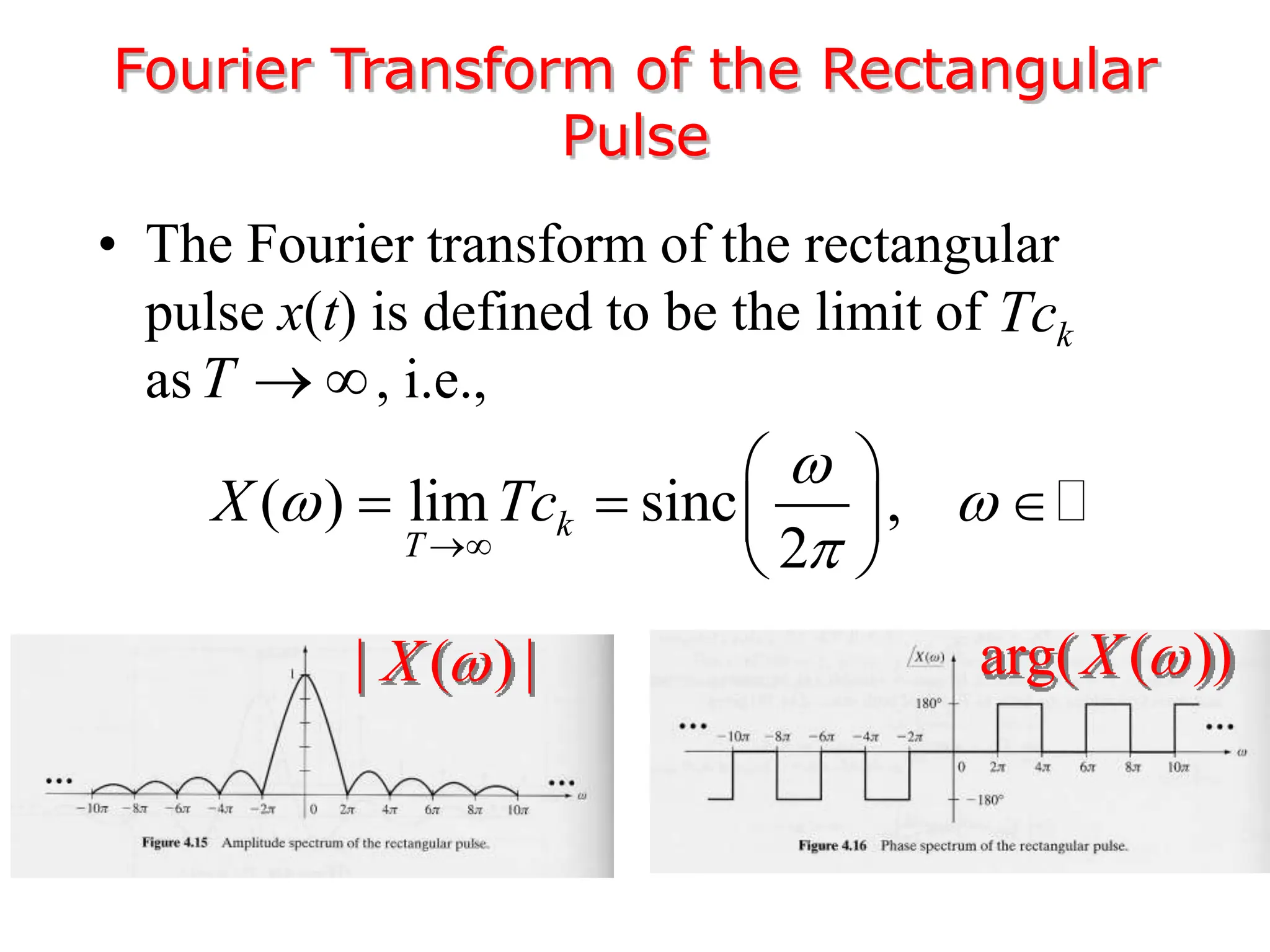
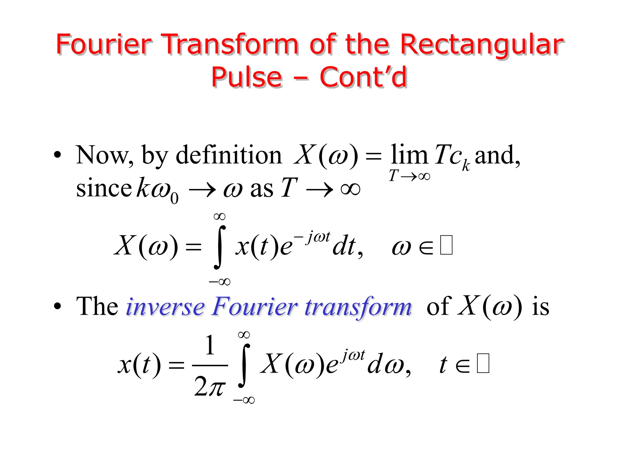
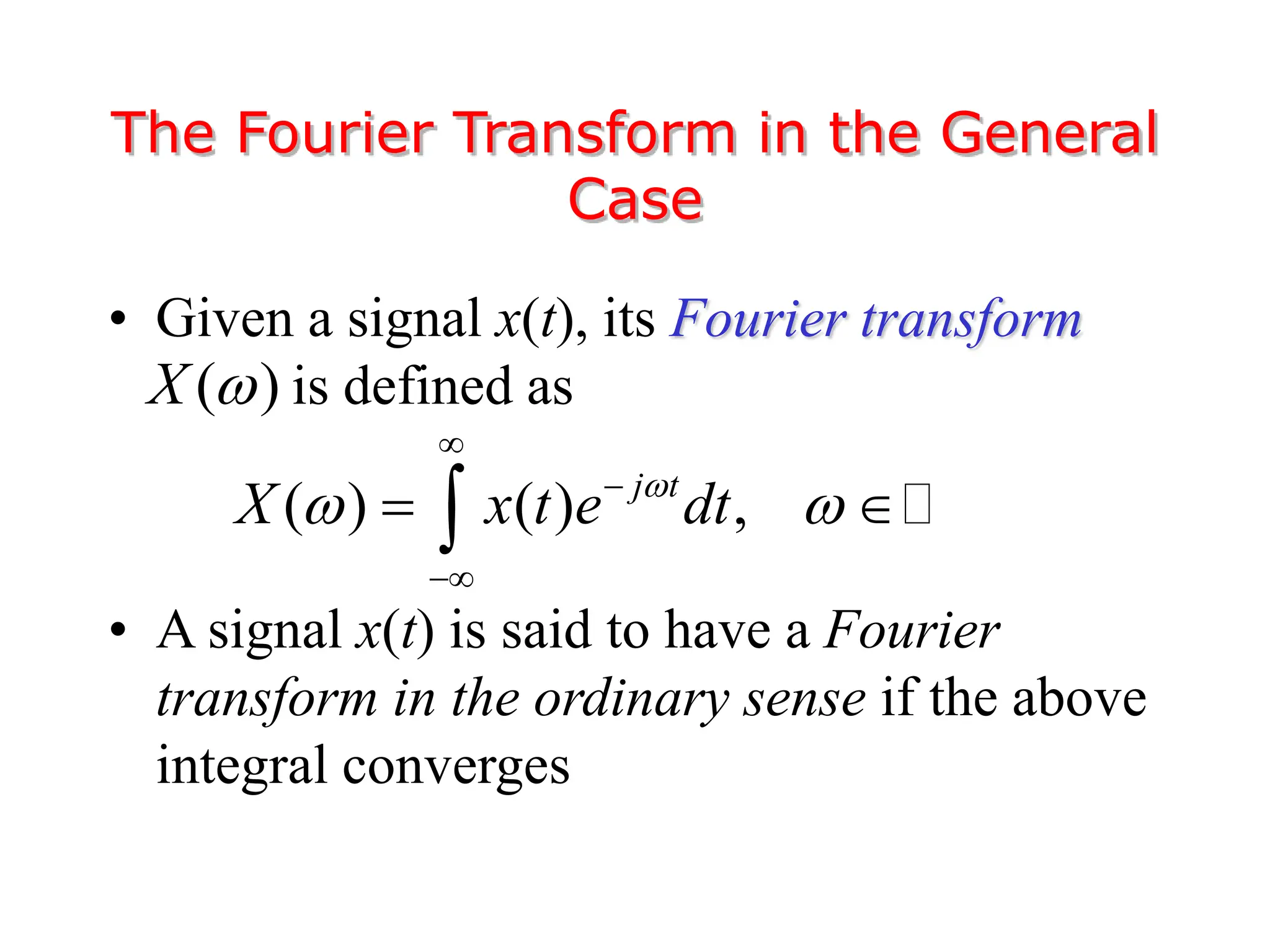
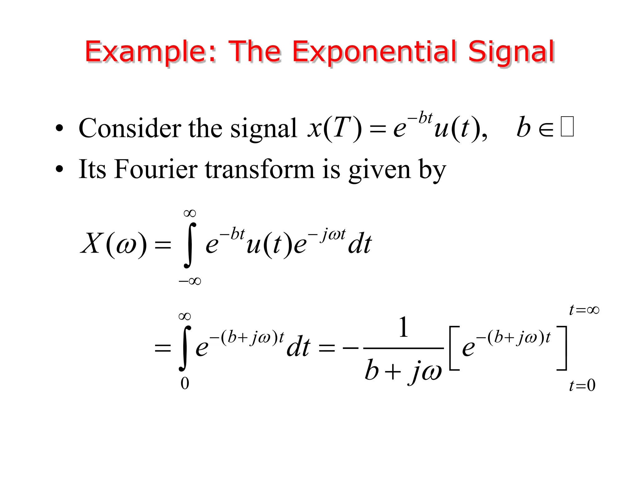
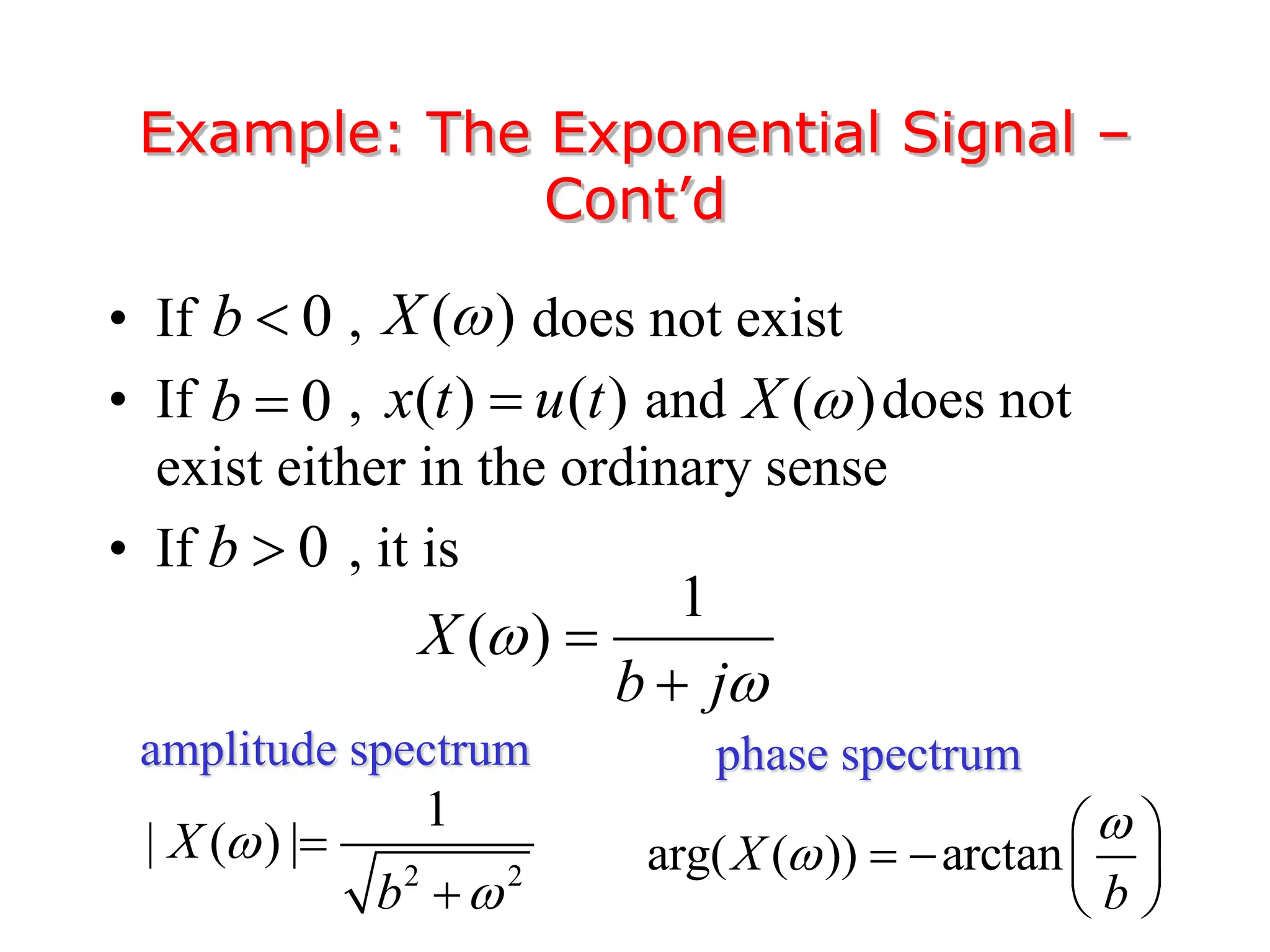
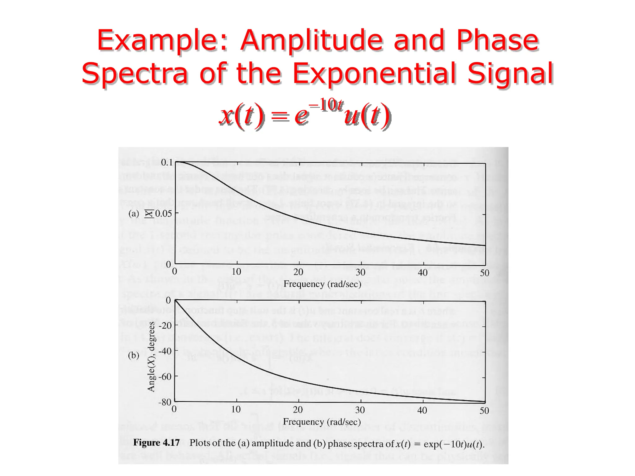
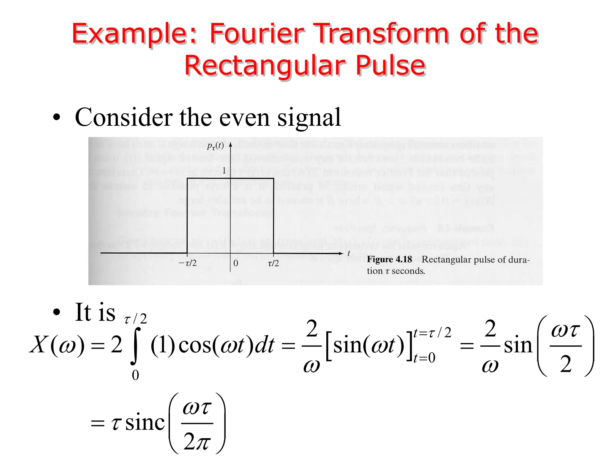
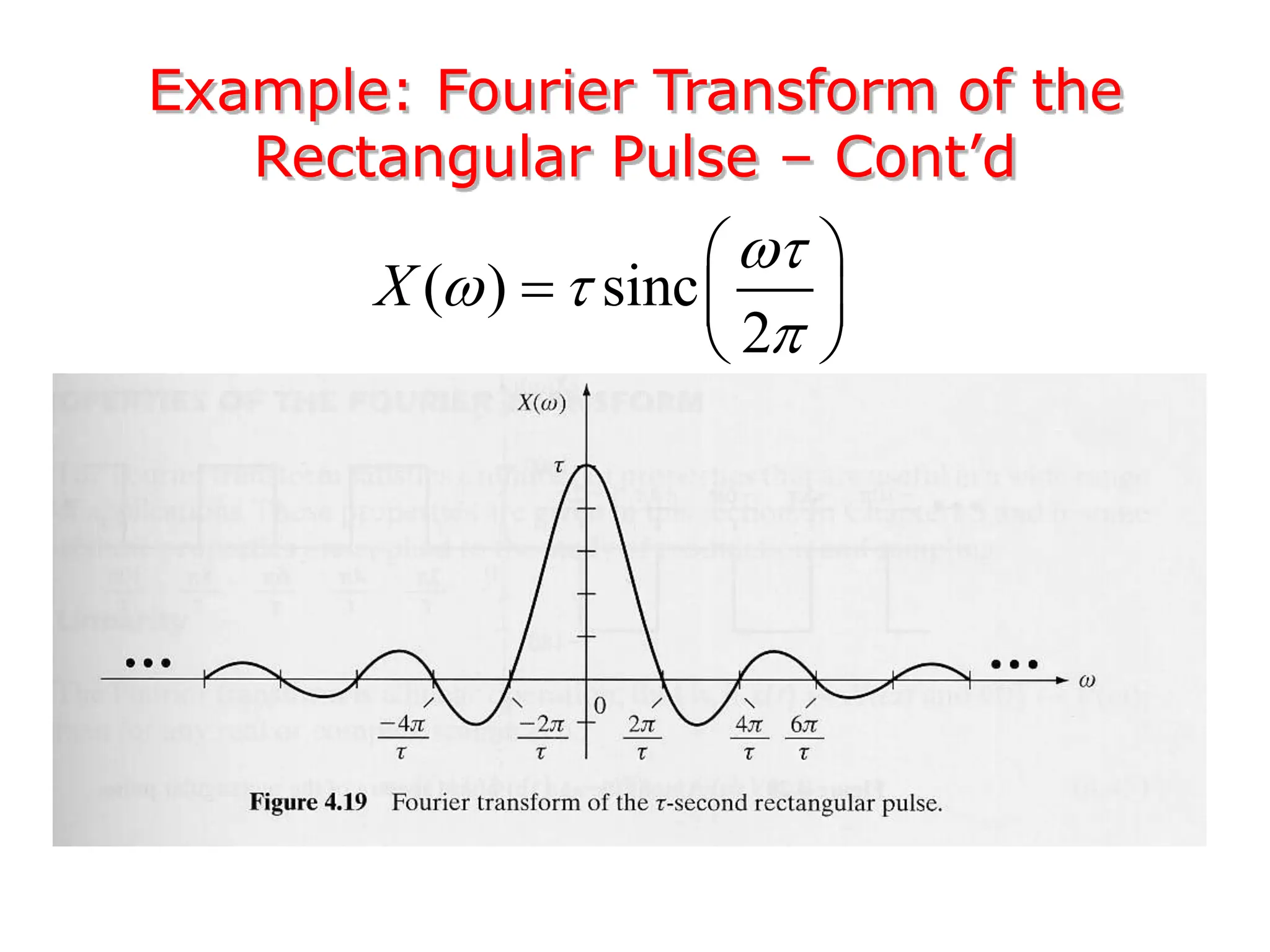
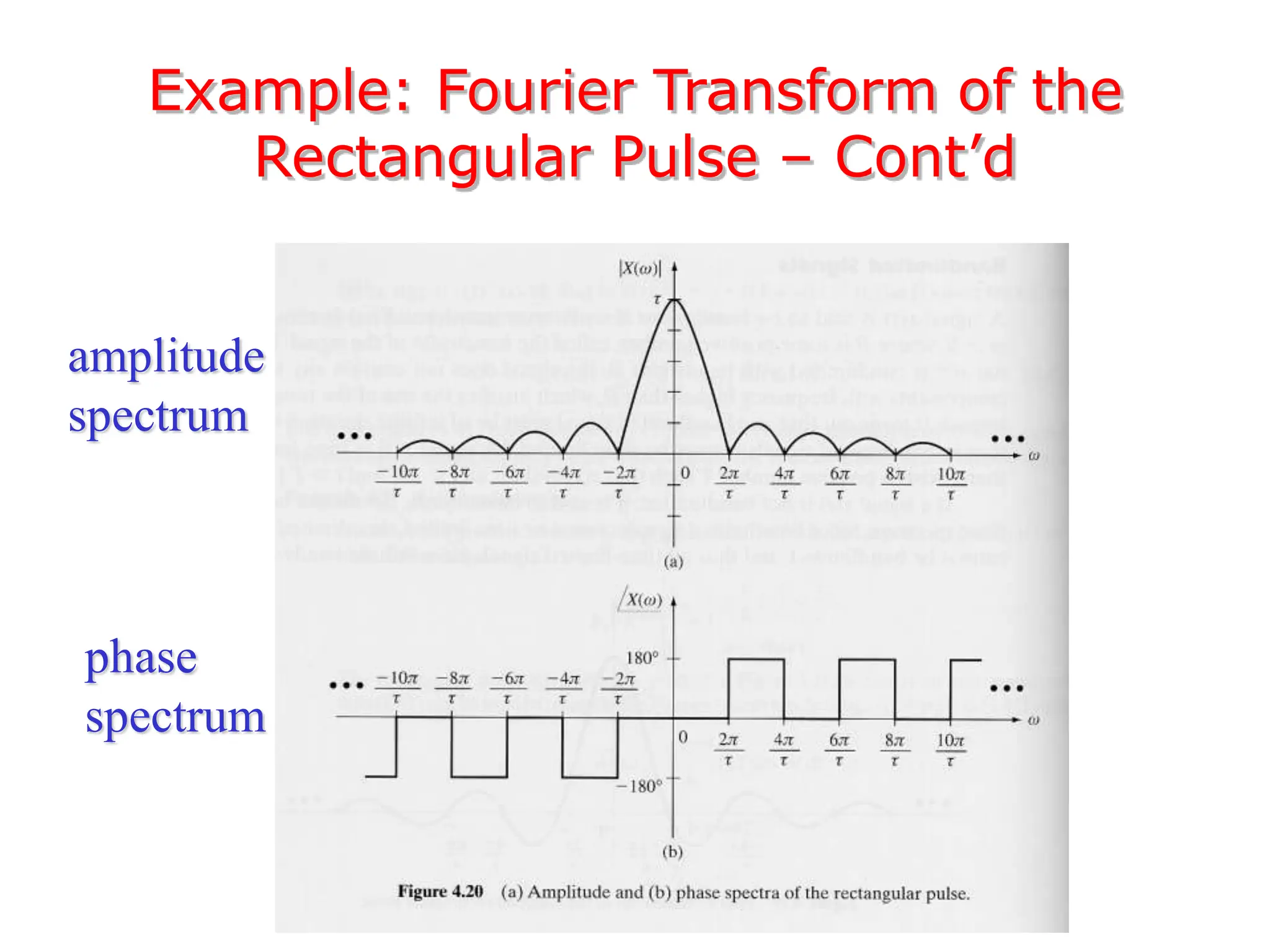
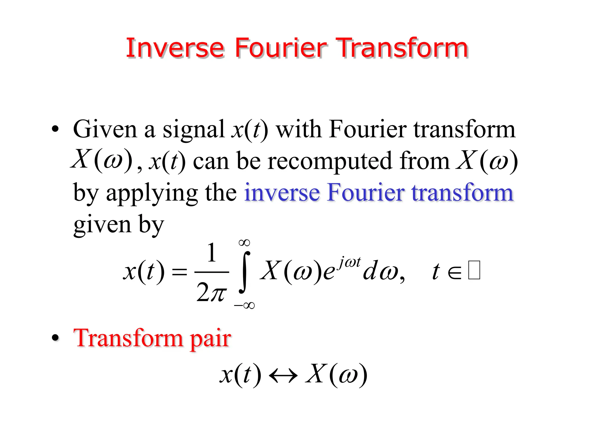
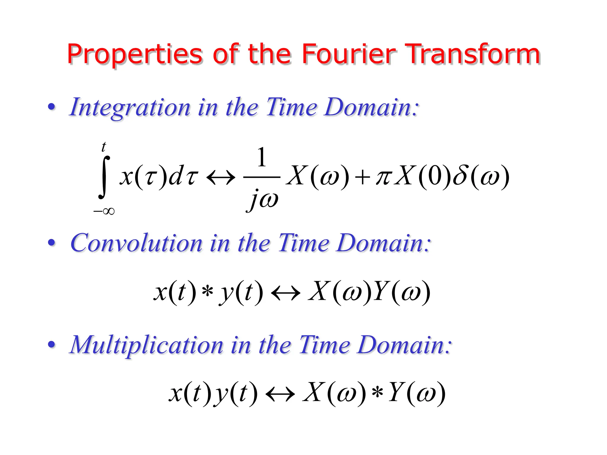
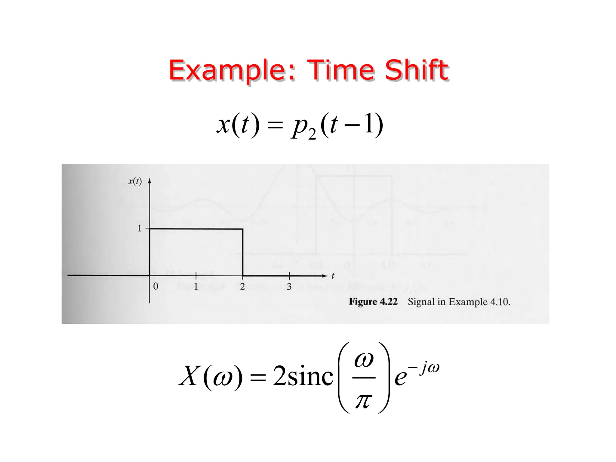
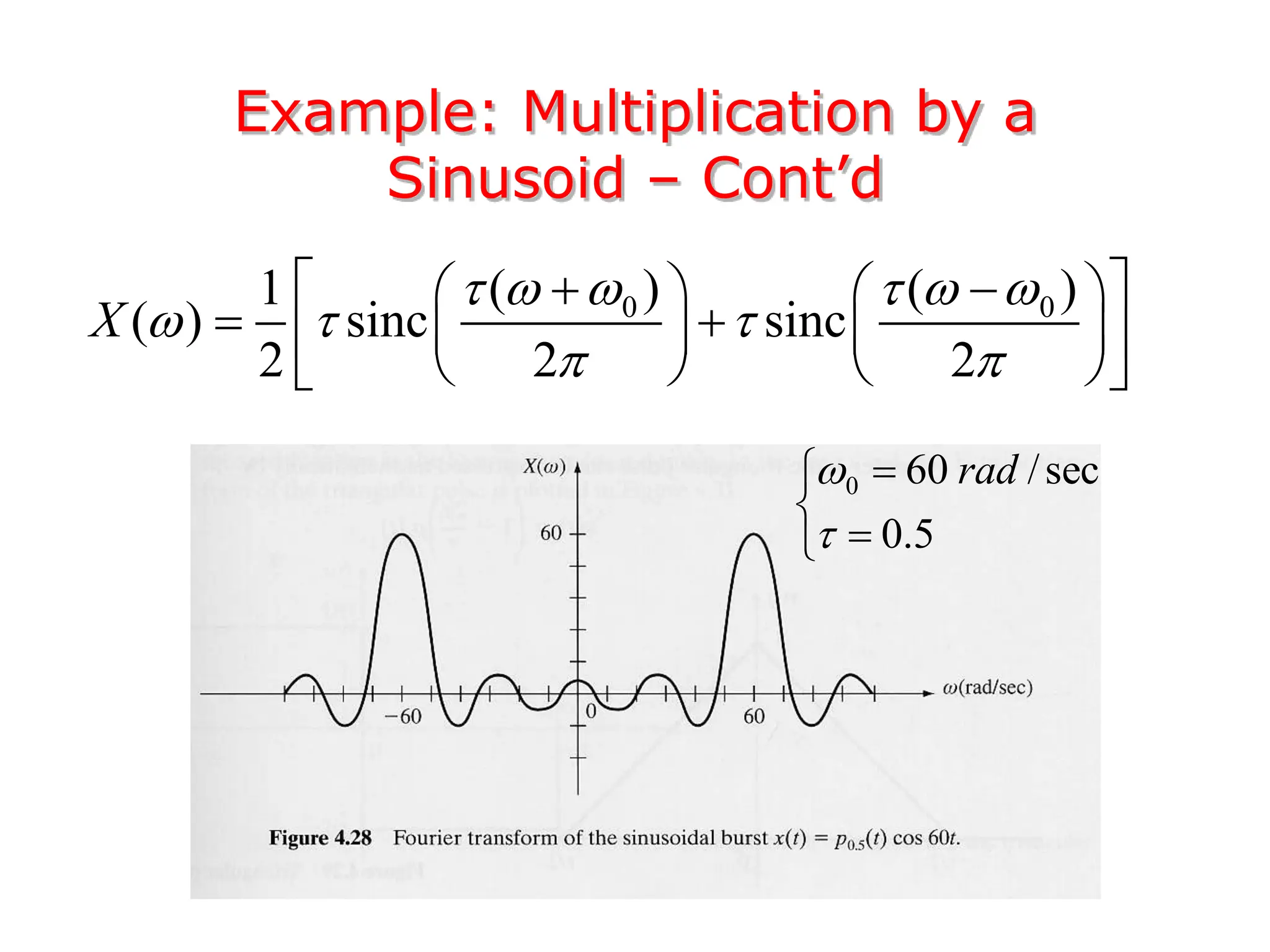
3. The Fourier transform allows representing aperiodic signals as a sum of sinusoids of all possible frequencies, resulting in a continuous spectrum rather than a discrete line spectrum. The Fourier transform of a rectangular pulse is a sinc function.

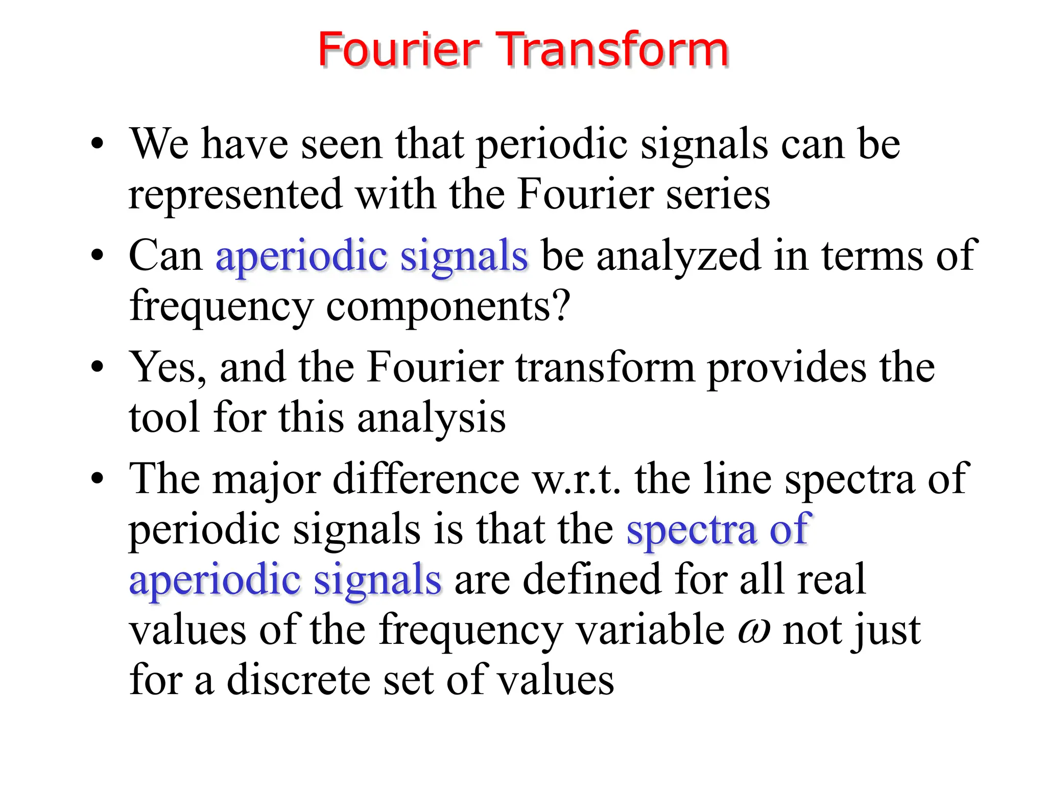
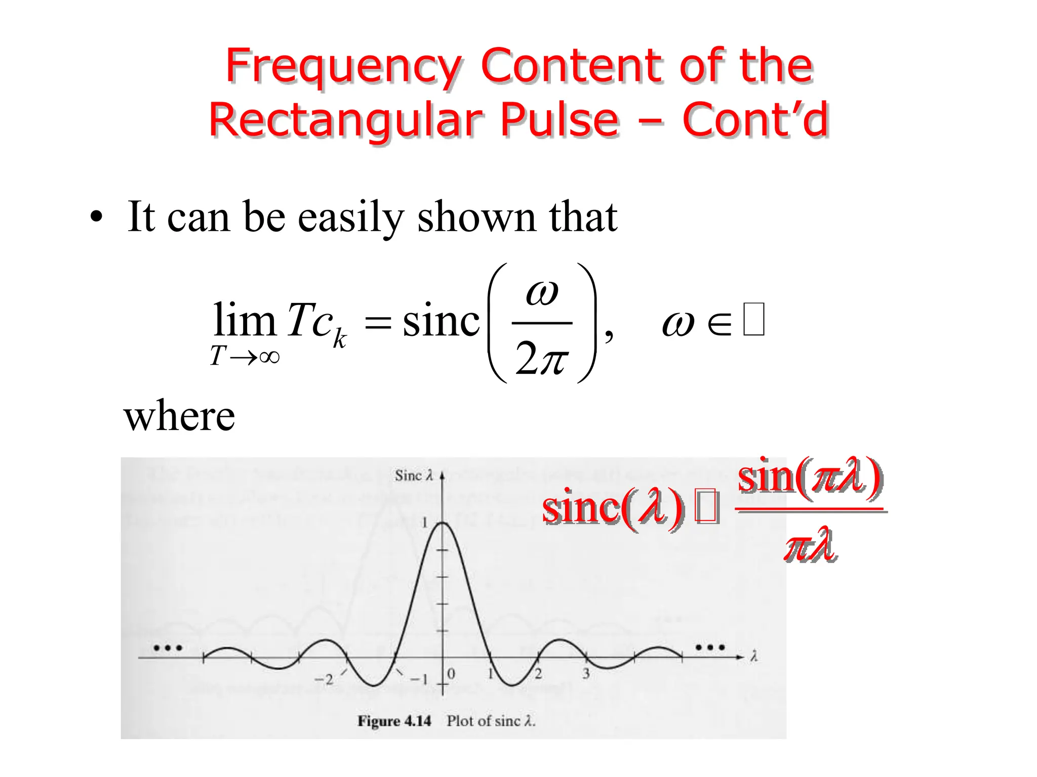


![Circuit Network Analysis - [Chapter4] Laplace Transform](https://cdn.slidesharecdn.com/ss_thumbnails/ch4-150613063858-lva1-app6891-thumbnail.jpg?width=640&height=640&fit=bounds)