Downloaded 285 times

![EE-2027 SaS, L2 3/25
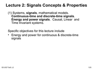
Reminder: Continuous & Discrete Signals
x(t)
t
x[n]
n
Continuous-Time Signals
Most signals in the real world are
continuous time, as the scale is
infinitesimally fine.
E.g. voltage, velocity,
Denote by x(t), where the time
interval may be bounded (finite) or
infinite
Discrete-Time Signals
Some real world and many digital
signals are discrete time, as they
are sampled
E.g. pixels, daily stock price
(anything that a digital computer
processes)
Denote by x[n], where n is an integer
value that varies discretely
Sampled continuous signal
x[n] =x(nk)](https://image.slidesharecdn.com/lecture2-131002071456-phpapp01/85/Lecture2-Signal-and-Systems-3-320.jpg)
![EE-2027 SaS, L2 4/25
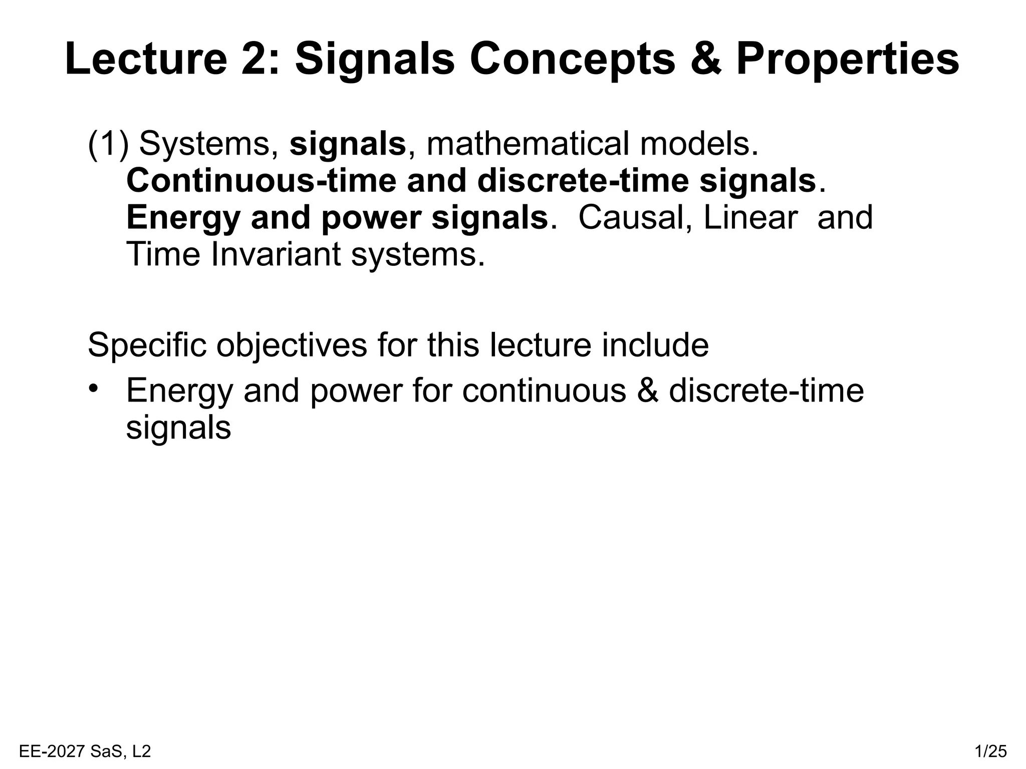
“Electrical” Signal Energy & Power
It is often useful to characterise signals by measures such
as energy and power
For example, the instantaneous power of a resistor is:
and the total energy expanded over the interval [t1, t2] is:
and the average energy is:
How are these concepts defined for any continuous or
discrete time signal?
)(
1
)()()( 2
tv
R
titvtp ==
∫∫ =
2
1
2
1
)(
1
)( 2
t
t
t
t
dttv
R
dttp
∫∫ −
=
−
2
1
2
1
)(
11
)(
1 2
1212
t
t
t
t
dttv
Rtt
dttp
tt](https://image.slidesharecdn.com/lecture2-131002071456-phpapp01/85/Lecture2-Signal-and-Systems-4-320.jpg)
![EE-2027 SaS, L2 5/25
Generic Signal Energy and Power
Total energy of a continuous signal x(t) over [t1, t2] is:
where |.| denote the magnitude of the (complex) number.
Similarly for a discrete time signal x[n] over [n1, n2]:
By dividing the quantities by (t2-t1) and (n2-n1+1), respectively,
gives the average power, P
∫=
2
1
2
)(
t
t
dttxE
∑ =
= 2
1
2
][
n
nn
nxE](https://image.slidesharecdn.com/lecture2-131002071456-phpapp01/85/Lecture2-Signal-and-Systems-5-320.jpg)
![EE-2027 SaS, L2 6/25
Energy and Power over Infinite Time
For many signals, we’re interested in examining the power and energy
over an infinite time interval (-∞, ∞). These quantities are therefore
defined by:
If the sums or integrals do not converge, the energy of such a signal is
infinite
Two important (sub)classes of signals
1. Finite total energy (and therefore zero average power)
2. Finite average power (and therefore infinite total energy)
Signal analysis over infinite time, all depends on the “tails” (limiting
behaviour)
∫∫
∞
∞−−
∞→∞ == dttxdttxE
T
T
T
22
)()(lim
∑∑
∞
−∞=−=∞→∞ == n
N
NnN nxnxE
22
][][lim
∫−
∞→∞ =
T
T
T dttx
T
P
2
)(
2
1
lim
∑ −=∞→∞
+
=
N
NnN nx
N
P
2
][
12
1
lim](https://image.slidesharecdn.com/lecture2-131002071456-phpapp01/85/Lecture2-Signal-and-Systems-6-320.jpg)
![EE-2027 SaS, L2 9/25
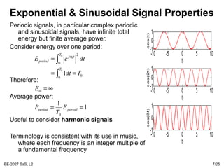
Discrete Unit Impulse and Step Signals
The discrete unit impulse signal is defined:
Useful as a basis for analyzing other signals
The discrete unit step signal is defined:
Note that the unit impulse is the first
difference (derivative) of the step signal
Similarly, the unit step is the running sum
(integral) of the unit impulse.
=
≠
==
01
00
][][
n
n
nnx δ
≥
<
==
01
00
][][
n
n
nunx
]1[][][ −−= nununδ](https://image.slidesharecdn.com/lecture2-131002071456-phpapp01/85/Lecture2-Signal-and-Systems-9-320.jpg)
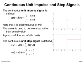


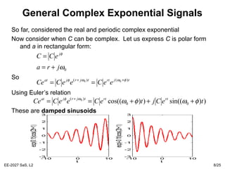
This document covers key concepts about signals including: 1) It defines continuous-time and discrete-time signals, and discusses the concepts of energy and power for both types of signals. 2) It provides the mathematical definitions of total energy, average power, and characterizes signals based on whether they have finite or infinite total energy and average power. 3) It discusses properties of exponential and sinusoidal signals, including that they have infinite total energy but finite average power. 4) It introduces common basic signals like the unit impulse and unit step signals in both continuous and discrete time.