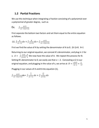
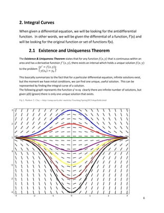
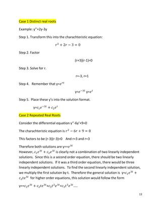
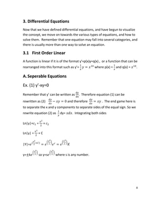
This document provides an overview of topics covered in a differential equations course, including: 1. Review of integration by parts and partial fractions. 2. Discussion of integral curves and the existence and uniqueness theorem for differential equations. 3. Classification and methods for solving first and higher order linear differential equations, including separable, exact, integrating factors, Bernoulli, homogeneous with constant coefficients, and undetermined coefficients. 4. Brief introduction to additional solution methods like Euler's method, power series, and Laplace transforms. 5. Mention of solving systems of linear differential equations.

1. 1
Embry-Riddle Aeronautical University, Prescott
MA345 – Differential Equations and Matrix Methods
Dr. Tsutsui, Hisaya
A summary by Adan Magaña
ERAU ID# 1424413

2. 2
Table of Contents
1. Review
1.1 Integration By Parts
1.2 Partial Fractions
2. Integral Curves
2.1 Existence and Uniqueness Theorem
2.2 Hard to solve Equations
3. Differential Equations
3.1 First Order Linear
A. Seperable
B. Exact
C. Integrating Factors
D. Bernoulli
3.2 Higher Order Linear
A. Homogenous with constant coeffecients
B. Undetermined Coeffecients

3. 3
4. Methods of Approximation
4.1 Euler
4.2 Huen
4.3 Power Series
5. Laplace Transforms
5.1 Derivation
5.2 Convolutions
5.3 Impulse
5.4 Delta Function
6. Systems of Linear Differential Equations

4. 4
I. REVIEW
Any responsible paper regarding Differential Equations would do well to review a
couple of concepts from previous courses in Mathematics. Two remedial
concepts that will appear throughout this course will be Integration by Parts, and
Partial Fractions. A thorough understanding of these concepts will aid the student
immensely.
1.1 Integration By Parts
Ex.
When integrating by parts, we first split the above equation into the two parts
and . We will choose one part to integrate, and one part to differentiate,
denoted below by the I and D columns, respectively. When choosing which part
to integrate, and which part to differentiate, we remember the mnemonic, LIPET.
This mnemonic represents the terms Log, Inverse, Polynomial, Exponent, and Trig,
where the terms on the left will always be differentiated and the terms on the
right will always be integrated. In this case, we have a polynomial and an
exponential. Since P comes before E in LIPET, we will differentiate and
integrate .
Paying close attention to the arrows and the (s)igns, we have
3
x
e x dx
x
e
3
x
3
x
x
e

5. 5
1.2 Partial Fractions
We use this technique when integrating a fraction consisting of a polynomial over
a polynomial of greater degree, such as
Ex. ∫( )( )
First separate the bottom two factors and set them equal to the entire equation
as follows.
(1) ∫ ( )
∫ ( )
= ∫ ( )( )
First we find the value of A by setting the denominator of A to 0. (X-1)=0. X=1
Returning to our original equation, we conceal A’s denominator, and plug in 1 for
x. ∫ ( )
= We now have the value of A. We repeat this process for B.
Setting B’s denominator to 0, we easily see that x = -2. Concealing x+2 in our
original equation, and plugging in the value of x, we arrive at .
Plugging in our values of A and B into equation (1),
∫ ( )( )
dx ∫ ( )
∫ ( )

6. 6
2. Integral Curves
When given a differential equation, we will be looking for the antidifferential
function. In other words, we will be given the differential of a function, f’(x) and
will be looking for the original function or set of functions f(x).
2.1 Existence and Uniqueness Theorem
The Existence & Uniqueness Theorem states that for any function ( ) that is continuous within an
area and has a derivative function ( ), there exists an interval which holds a unique solution ( )
to the problem {
( )
( )
}.
This basically summarizes to the fact that for a particular differential equation, infinite solutions exist,
but the moment we have initial conditions, we can find one unique, useful solution. This can be
represented by finding the integral curve of a solution.
The following graph represents the function y’=x-xy clearly there are infinite number of solutions, but
given y(0) (green) there is only one unique solution that exists.
Fig 2. Mathew T. Clay -- http://comp.uark.edu/~mattclay/Teaching/Spring2013/slopefields.html

7. 7
2.2 Hard to solve functions
In addition to helping the student visualize the uniqueness theorem,
Integral curves often help to visualize functions that might otherwise be
difficult to solve.
Ex. y’=x-y+1
C=x-y+1
y=x+1-c
c= -2: y=x+3
c= -1: y=x+2
c= 0: y=x+1
c= 1: y=x
c= 2: y=x-1

8. 8
3. Differential Equations
Now that we have defined differential equations, and have begun to visualize
the concept, we move on towards the various types of equations, and how to
solve them. Remember that one equation may fall into several categories, and
there is usually more than one way to solve an equation.
3.1 First Order Linear
A function is linear if it is of the format y’+p(x)y=q(x) , or a function that can be
rearranged into this format such as y’+ where p(x) = and q(x) = .
A.Seperable Equations
Ex. (1) y’-xy=0
Remember that y’ can be written as . Therefore equation (1) can be
rewritten as (2) and therefore . The end game here is
to separate the x and y components to separate sides of the equal sign. So we
rewrite equation (2) as dy= . Integrating both sides
Ln|y|+ = +
Ln|y| = + C
|Y|= ( ) ( ) ( )
y= k
( )
so y=s
( )
where s is any number.

9. 9
B. Exact
An exact equation is one that holds the form M(xy)dx+N(xy)dy=0.
where
( )
=
( )
Ex. ( ) ( )
M(xy)=4x N(xy)=4x
4x=4x, so this equation is exact.
Now that we have identified this solution as an exact solution, we can set out to
solve it.
Let ( ) and let ( ) .
F(xy)=the integral of with respect to x.
(1) F(xy) = + g(y).
We now have the form of the integral, but we need to find the value of g(y). We
find this value by differentiating. Since we integrated with respect to x, we will
differentiate with respect to y.
(2) (xy) =2 ( )
Note that this is very similar to N(xy). If this is not the case, it is probable that an
Integration error was made, or that the problem is not exact.
Setting this equal to N(xy):
(3) 2 ( )
It is obvious that g’(y) is equal to 2y. g(y) must then be equal to .
Plugging this value into equation number one, our solution is
F(xy) = + .

10. 10
C. Integrating Factors
Returning to the problem at the beginning of section 3.1
Eq.1 y’+ where p(x) = and q(x) = We will multiply each term in
this equation by an Integrating factor so that the equation becomes
Eq 2. (IF)y’+(IF) ( ) . Using some Japanese Ninja magic taught in
Ma345, * we know that this reduces to
Eq. 3 (IF)y’=(IF) To solve for the Integrating factor, we raise e to the integral
of p(x). In this case, the Integrating Factor is ∫
= ( )
=x. Multiplying this IF
through the equation 3 xy’ = . Thus y’= and y= .
*Actually, this reduction can be shown through the use of µ(x) and an example of
this is found on page 49 of the course textbook.

11. 11
D.Bernoulli
An equation of the form +P(x)y=Q(x) is called a Bernoulli Differential
Equation where n does not equal zero or one.
y’=p(x)y+q(x) where n does not equal zero or one.
( )
+q(x)
Example:
-1
Let u = and u’=(1-n) ( )( )
For our example, u= and u’ =
u’+
Note that in this format we can use the integrating factors method we learned in
Section 3:4.
IF= ∫
xu’=x
xu=∫
u=
since y=1/u we substitute in those values and arrive at .

12. 12
3.2 Higher Order Linear
It is at this point that we are reminded of the Basic Existence Theorem. We have
already dealt with Differential equations of the first order. We now turn our
attention to the nth order linear circuits where n is greater than one.
A.Homogenous with constant coefficients
Characteristic equation
Ex. y’’+Ay’+By=0
Let y=
then y’ =
and y’’=
Substituting these values into our example,
+A +B =0
This simplifies to . This is known as the characteristic equation.
Although it is helpful to see how the characteristic equation is derived, this
transformation is often done directly without converting and factoring.
Solution Format
It is important to remember that if are both solutions, then is
a solution. Additionally, every multiple of this solution is also a solution.
Therefore, the solution will take the form of
y=

13. 13
Case 1 Distinct real roots
Example: y’’+2y-3y
Step 1. Transform this into the charachteristic equation:
Step 2. Factor
(r+3)(r-1)=0
Step 3. Solve for r.
r=-3, r=1
Step 4. Remember that y=
y= y=
Step 5. Place these y’s into the solution format.
y=
Case 2 Repeated Real Roots
Consider the differential equation y’’-6y’+9=0
The charachteristic equation is
This factors to be (r-3)(r-3)=0 And r=3 and r=3
Therefore both solutions are y==
However, is clearly not a combination of two linearly independent
solutions. Since this is a second order equation, there should be two linearly
independent solutions. If it was a third order equation, there would be three
linearly independent solutions. To find the second linearly independent solution,
we multiply the first solution by t. Therefore the general solution is y=
for higher order equations, this solution would follow the form
y== + + …..

14. 14
Case 3. Conjugate Complex Roots
The two cases noted above are for the equations which factor into base roots.
At times, the charachterstic will not factor evenly, and will require the use of
the quadratic formula thus ending in the roots a bi. Therefore y= ( )
( )
. These are complexfunctions, and it is often desireable to have two
real functions. Recall Euler’s formula
We use this to arrive at ( )for the two separate roots
a bi.
Example: y” +y=0.
Step 1. Characteristic equation
Step 2. Factor. r=0±i
Step 3. Format using Euler’s formula y= ( )
Initial Values.
We have already looked at general solutions for various types of homogenous
differential equations. Now we will consider Homogenous equations with
initial values. Assuming the initial values of y(0)=0 and y’(0)=1 in the equation
y’’+y=0.
We previously found this general solution to be
Eq 1.y= ( ).
Eq 2 y’= ( ).
Plugging in our initial conditionsfor y’ into Eq 2. ( ).
Applying initial condition y(0)=0 to Eq 1.
0=( )
The unique solution becomes y=sin(t)

15. 15
B Homogenous Equations with Undetermined
Coeffecients
These take the form of the characteristic equation set equal to some f(x).
Example: y’’+2y’-3y=2
This solution will take the form y= where y is the general homogenous
solution as found in the previous section, and is a particular integral.
A careful observer will note that this equation is very similar to the example
used above in “Case 1. Distinct real roots”
We first set this equation equal to zero, and solve for the homogenous
equation. As found above
Now we will find the particular Integral of f(x) of the form A
Step 1. Since this is an equation of the second order, we will find and .
4 A and 16 A
Step 2. Substitute these values into the original equation.
16 A +2(4 A )-3 A 2
21 A =2
Step 3. Solve for A
A=
Step 4. Substitute this value into A for
Since y=
y=

16. 16
4.Methods of Approximation
4.1 Euler’s Method
This method is relatively simple, but not very accurate. It will be used as a
basis for a more complex, more accurate method, so understanding of this
method is vital before moving on.
Consider the following Euler Table for the function ( )
With h=0.1 , y(0)=1, evaluated at x=0.4
Notice that ( ) from the same row.
Also notice that . In other words, the x value is equal to h times
the value of the n in the row above it.
( ) This can be more easily understood that the y
value in any row is equal to the value of the y value above it plus the value in the
last column in the row above it.
n xn yn f(xnyn) hf(xnyn)
0 0 1 -1 -1
1 0.1 0.9 -0.8 -0.08
2 0.2 0.82 -0.6324 -0.06324
3 0.3 0.7568 -0.4827 -0.04827
4 0.4 0.7085 -0.34202

17. 17
4.2 Huen’s Method
Now let us consider the same function, this time approximated with
Huen’s method.
( )
Where h=0.1, y(0)=1, x(0)=0, evaluated at x=0.4
You will notice that this graph is similar to the one used in Euler’s method, with
the exception of the last column. You will also notice that the in that
column does not correspond to the value of y in the row below it.
Remember in this method that (xn+1, yn+1) = (xn + h, yn + h f(xn, yn))
n xn yn f(xnyn) hf(xnyn) yn+1
0 0 1 -1 -1
1 0.1 0.91 -0.8181 -0.08181 0.9
2 0.2 0.8368 -0.6602 -0.06602 0.82819
3 0.3 0.7786 -0.5162 -0.05162 0.77078
4 0.4 0.7344 -0.34202 0.72698

18. 18
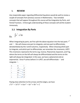
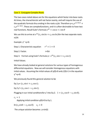
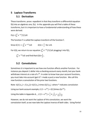
4.3 Power Series
When given an equation such as
EX. y”-y’+2xy=x+
where y(0)= and y’(0) =
Step 1. Arrange formula to solve for y”
y”=x+ -2xy+y’
Step 2. Insert initial conditions
y”(0)=1+=
Step 3. Take derivitave of y”
y”’=1+ -2y-2xy’=y”
Step 4. Insert initial conditions
y”’(0)=3-2 +3
Step 5. Insert values into the formula below ( )
( ) ( ) ( )
+ ...
Step 6. Combine like terms
y= + + + ]+[ + + ]

19. 19
5 Laplace Transforms
5.1 Derivation
These transforms prove expedient in that they transform a differential equation
f(t) into an algebraic one, f(s). In the appendix you will find a table of these
transforms, but it is important to have a fundamental understanding of how these
were derived.
F(s) =∫ ( )
The function F is called the Laplace transform of the function f.
Since ( ) ∫ £(1) = for s>0.
For £(t), we return to our equation ∫ ( ) plugging t into f(t),
∫ and find that £(t)= .
5.2 Convolutions
Sometimes it is important to see how one function affects another function. For
instance you deposit 1 dollar into a checking account every month, but your bank
withdraws interest at a rate of . In order to know how your account functions,
you must take into account (get it? I made a pun) a new function. We call this
new function a convolution of the prior two functions.
Note- £( ( ) ( ))= £( ( ) times £( ( ) where * indicates convolution
Using our bank account example, £ ( ) = £( )times £( ).
Using the table in Appendix A, , £ ( ) = =
( )
However, we do not want the Laplace of this convolution, we want the
convolution itself, so we now take the Laplace inverse of both sides. Using Partial

20. 20
fractions, £ ( ) = Laplace inverse ( ). Using the Laplace table, we find
the solution to our convolution to be + .
5.3 Impulse
The step function is used throughout engineering. In the field of Electrical
Engineering, it represents a switch. When time is less than 0, the power is
off. When time is greater than zero, the switch closes, and power is turned
on. Since this provides a non-continuous function, it would prove difficult
to solve using normal methods of solving differential equations. The
Laplace transforms make this solution quite straightforward and simple.
To find the Laplace of the step function where voltage goes from 0 volts at
time to 5 volts when a switch is flipped at time zero, we consider:
£( ( )) This can also be written as £(u(t-5)) which clearly becomes .
5.4 Delta Function
Now that we have discussed the step function, often called the impulse
function, we have laid the groundwork to discuss the Dirac Delta Function.
Put simply, the dirac delta function denoted as is equal to the limit as h
approaches zero of uh(t) over h.
Example. y”+y= (t- )
y(0)=1, y’(0)=0
ℒ(y”+y’)= ℒ ( (t- )
ℒ(y”)+ ℒ(y’)= .
ℒ(y)=
y= cos(t)+u(t-- )sin(t-- )

21. 21
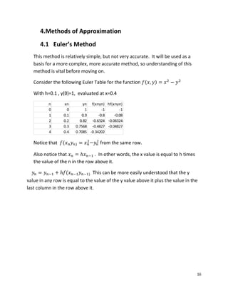
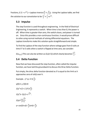
6 Systems of Linear Differential Equations
A system of LD equations is any set of equations such that some x=f(t),
y=g(t) simultaneously satisfies both equations of the system.
Example:y”-3y’+2y=
= y, =y’
= ,
Place these two equations into matrix form.
[ =[ ] [ ]+[ ] where A is [ ]
The characteristic format of A
is[ ]
Step 1. Set the determinant of the characteristic equation of A =0 and solve for .
( )( ) =0
( )( )=0
Step 2. Apply the lambda values found in Step 1 into the characteristic form of A
For ,
[ ] [ ]=[ ]
For ,
[ ] [ ]=[ ]
[ ]=[ ] [ ]

22. 22
Appendix A
Formuals
Quadratic formula
√
Important formula used to go from Euler’s to a useful real number
( )

23. 23
Appendix B Laplace Table

24. 24
Final Note:
You may notice that Jones and I have the same image for the graph in section
2:1. It is important for me to point out that while struggling to graph these
curves on one of our programming platforms, I asked for his help. He told me
he used the internet. There seemed to be a shortage of images that displayed
what I hoped to point out, and so I used the same picture. He had it first.