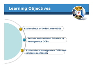
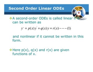
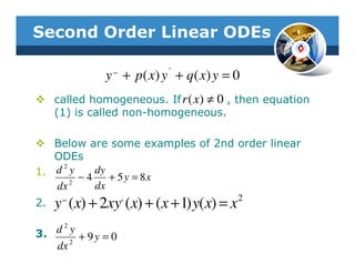
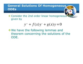
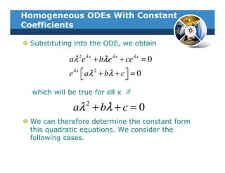
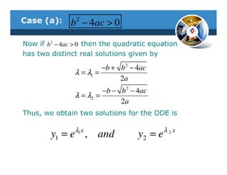
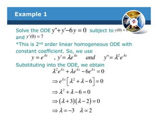
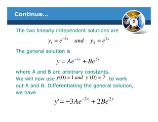
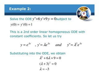
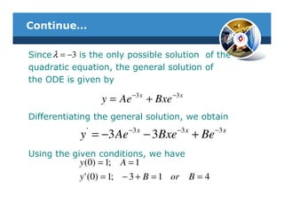
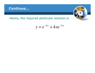
This document provides an overview of engineering mathematics II, specifically focusing on second order ordinary differential equations (ODEs). It defines linear and nonlinear second order ODEs and discusses the general solutions of homogeneous ODEs. It also examines homogeneous ODEs with constant coefficients, providing examples and discussing different cases based on the characteristic equation. The document concludes by solving sample second order linear homogeneous ODEs with constant coefficients.

1. KNF1023
Engineering
Mathematics II
Second Order ODEs
Prepared By
Annie ak Joseph
Prepared By
Annie ak Joseph Session 2008/2009

2. Learning Objectives
Explain about 2nd Order Linear ODEs
Discuss about General Solutions of
Homogeneous ODEs
Explain about Homogeneous ODEs with
constants coefficients

3. Second Order Linear ODEs
A second-order ODEs is called linear if it
can be written as
,, '
y + p ( x) y + q ( x) y = r ( x) − − − (1)
and nonlinear if it cannot be written in this
form.
Here p(x), q(x) and r(x) are given
functions of x.

4. Second Order Linear ODEs
,, '
y + p ( x) y + q ( x) y = 0
called homogeneous. If r ( x ) ≠ 0 , then equation
(1) is called non-homogeneous.
Below are some examples of 2nd order linear
ODEs
2
1. d y − 4 dy + 5 y = 8 x
dx 2 dx
,, , 2
2. y (x) + 2xy (x) + (x + 1) y(x) = x
3. d2y
2
+ 9y = 0
dx

5. General Solutions Of Homogeneous
ODEs
Consider the 2nd order linear homogeneous ODE
given by
,, ,
y + f ( x) y + g ( x) y = 0
We have the following lemmas and
theorem concerning the solutions of the
ODE.

6. Lemma #1, #2 and Theorem 2
Lemma #1
If y1 (x ) and y 2 ( x ) are solutions of the above
ODE (over a certain interval), then y(x) = Ay1 (x) + By2 (x)
where A and B are any arbitrary constants, is
also a solution of the ODE (over the interval).
Lemma# 2
If y 1 ( x ) and y 2 ( x ) are solutions of the above 2nd
order linear homogeneous ODE, then
'
2 1
'
1 2 (
y y − y y = D exp − ∫ f ( x ) dx )
where D is a constant

7. Theorem 2
If y1 (x ) and y 2 ( x ) are solutions of the above
2nd order linear homogeneous ODE (over a
certain interval) and if y1 (x ) and y 2 ( x ) are linearly
independent of each other (over the interval),
then the general solution of the ODE is given by
y( x ) = Ay1 ( x ) + By 2 ( x )
where A and B are arbitrary constants.

8. Homogeneous ODEs With Constant
Coefficients
A 2nd order linear homogeneous ODE with
constant coefficients is one which can be written
in the form
ay ( x ) + by ( x ) + cy ( x ) = 0
'' '
Here a ≠ 0, b and c are given constants.
According to Theorem #2, to construct the
general solution of the ODE, we have to
find any two linearly independent solutions
of the ODE.

9. Homogeneous ODEs With Constant
Coefficients
To look for a solution of the ODE, let us try
y ( x ) = eλ x
Where λ is a constant
Differentiating, we obtain
y '( x) = λ eλ x
y "( x) = λ ⋅ λ eλ x = λ 2 eλ x

10. Homogeneous ODEs With Constant
Coefficients
Substituting into the ODE, we obtain
aλ 2 eλ x + bλ eλ x + ceλ x = 0
 aλ 2 + bλ + c  = 0
λx
e  
which will be true for all x if
2
aλ + bλ + c = 0
We can therefore determine the constant form
this quadratic equations. We consider the
following cases.

11. Case (a): 2
b − 4ac > 0
Now if b 2 − 4ac > 0 then the quadratic equation
has two distinct real solutions given by
−b + b 2 − 4ac
λ = λ1 =
2a
−b − b 2 − 4ac
λ = λ2 =
2a
Thus, we obtain two solutions for the ODE is
λ1 x λ2x
y1 = e , and y2 = e

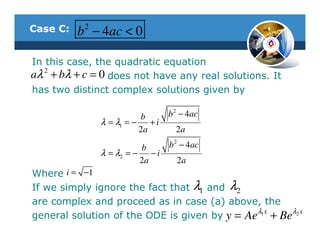
12. Continue…
y1 eλ1 x
= λ 2 x = e[ 1 2 ] ≠ cons tan t ,since λ1 ≠ λ2 .
λ −λ x
Now
y2 e
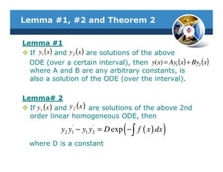
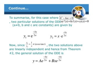
Hence, the two solutions are linearly
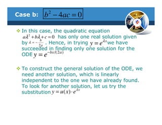
independent. For this case where b 2 − 4 ac > 0
from Theorem #2, the general solution of the
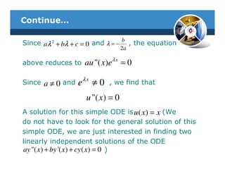
ODE ay "+ by '+ cy = 0 (a≠0, b, and c are constants)
is given by
λ1 x λ2 x
y = Ae + Be
where A and B are arbitrary constants and λ1 and λ2
are the solutions of the quadratic equation
2
aλ + bλ + c = 0

13. Example 1
Solve the ODE y"+ y '−6 y = 0 subject to y (0) = 1
and y ' (0) = 7
*This is 2nd order linear homogeneous ODE with
constant coefficient. So, we use
λx λx 2 λx
y=e , y ' = λe and y" = λ e
Substituting into the ODE, we obtain
λ 2 e λ x + λ e λ x − 6e λ x = 0
⇒e  λ 2 + λ − 6  = 0
λx

⇒ λ2 + λ − 6 = 0
⇒ ( λ + 3)( λ − 2 ) = 0
⇒ λ = −3 λ = 2

14. Continue…
The two linearly independent solutions are
−3 x 2x
y1 = e and y2 = e
The general solution is
−3 x 2x
y = Ae + Be
where A and B are arbitrary constants.
We will now use y ( 0 ) = 1 and y ' ( 0 ) = 7 to work
out A and B. Differentiating the general solution,
we have
−3 x 2x
y ' = −3 Ae + 2 Be

15. Continue…
So, y (0) = 1; A + B = 1
y ' (0) = 7; − 3 A + 2 B = 7
Solving for A and B, we obtain A = −1 and B = 2
Thus, the required particular solution of the ODE
is
−3 x 2x
y = −e + 2e

16. 2
Case b: b − 4ac = 0
In this case, the quadratic equation
aλ 2 + bλ + c = 0 has only one real solution given
b
by λ =−
2a
. Hence, in trying y = eλ x we have
succeeded in finding only one solution for the
− bx /(2 a )
ODE y = e
To construct the general solution of the ODE, we
need another solution, which is linearly
independent to the one we have already found.
To look for another solution, let us try the
λx
substitution y = u ( x ) ⋅ e

17. Continue…
where u ( x ) is a function to be determined.
Differentiating, we obtain
λx λx
y ' = λu ( x) ⋅ e + u '( x) ⋅ e
y '' = λ 2u ( x) ⋅ eλ x + 2λu '( x) ⋅ eλ x + u "( x)eλ x
Substituting into the ODE, we have
( ) ( )
a λ2u(x) ⋅ eλx + 2λu '(x) ⋅ eλx + u"(x)eλx + b λu(x) ⋅ eλx + u '(x) ⋅ eλx + cu(x)eλx = 0

18. Continue…
b
Since aλ 2 + bλ + c = 0 and λ = − , the equation
2a
λx
above reduces to au "( x)e =0
λx
Since a≠0 and e ≠0 , we find that
u "( x ) = 0
A solution for this simple ODE is u ( x ) = x (We
do not have to look for the general solution of this
simple ODE, we are just interested in finding two
linearly independent solutions of the ODE
ay "( x ) + by '( x ) + cy ( x ) = 0 )

19. Continue…
To summarise, for this case where b 2 − 4ac = 0
, two particular solutions of the ODEay "(x) + by '(x) + cy(x) = 0
(a≠0, b and c are constants) are given by
− bx − bx
y1 = e 2a
y2 = x ⋅ e 2a
y1 1
Now, since y2 = x ≠ (co ns tan t ) , the two solutions above
are linearly independent and hence from Theorem
#2, the general solution of the ODE is
− bx − bx
y = Ae 2a
+ Bxe 2a

20. Example 2:
Solve the ODE y"+6 y '+9 y = 0subject to
y ( 0) = y ' ( 0 ) = 1
This is a 2nd order linear homogeneous ODE with
constant coefficients. So let us try
y = e λx , y ' = λ e λx and y" = λ2 e λx
Substituting into the ODE, we obtain
λ 2 + 6λ + 9 = 0
(λ + 3) 2 = 0
λ = −3

21. Continue…
Since λ = −3 is the only possible solution of the
quadratic equation, the general solution of
the ODE is given by
−3 x −3 x
y = Ae + Bxe
Differentiating the general solution, we obtain
' −3 x −3 x −3 x
y = −3 Ae − 3Bxe + Be
Using the given conditions, we have
y (0) = 1; A =1
y ' (0) = 1; − 3 + B = 1 or B=4

22. Continue…
Hence, the required particular solution is
−3 x −3 x
y=e + 4 xe

23. Case C: b 2 − 4ac < 0
In this case, the quadratic equation
aλ 2 + bλ + c = 0 does not have any real solutions. It
has two distinct complex solutions given by
b b 2 − 4ac
λ = λ1 = − + i
2a 2a
b b 2 − 4ac
λ = λ2 = − −i
2a 2a
Where i = −1
If we simply ignore the fact that λ1 and λ2
are complex and proceed as in case (a) above, the
λx λ x
general solution of the ODE is given by y = Ae 1 + Be 2

24. Continue…
Theory which will be useful to us in dealing
λx
with e when λ is complex.
1. If z and w are any numbers (either real or
complex) then e z + w = e z ⋅ e w
2. If x is any real number then
± ix
e = cos( x) ± i sin( x)

25. Example 3
Solve the ODE y ' '−4 y '+13 y = 0 subject to
y (0) = 1 and y ' (0) = 2 . What is the value of y at
π
x= ?
2
This is 2nd order linear homogeneous ODE with
constant coefficients. Let us try
y = e λx , y ' = λ e λx and y" = λ 2 e λx
Substituting into the ODE, we obtain
λ2 − 4λ + 13 = 0
λ = 2 + 3i λ = 2 − 3i

26. Continue…
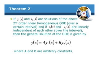
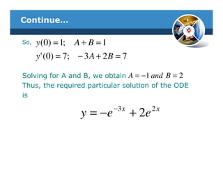
Thus, the general solution is given by
y = Ae ( 2+3i ) x + Be ( 2−3i ) x
Before we proceed any further, it is useful to
Rewrite the general solution as
(2 + 3i ) x (2 −3i ) x
y = Ae + Be
2x i (3 x ) − i (3 x )
y = e ( Ae + Be )
y = e 2 x ( A [ cos(3 x) + i sin(3 x) ] + B [ cos(3 x) − i sin(3 x) ])
y = e 2 x ([ A + B ] cos(3 x) + i [ A − B ] sin(3 x) )

27. Continue…
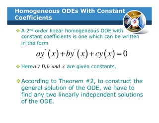
Thus, we can rewrite the general solution as
y = e 2 x [C cos(3 x) + D sin(3 x) ]
where C=A+B and D=i[A-B] are arbitrary
constants.
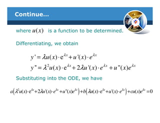
Differentiating, we have
y ' = e 2 x [− 3C sin(3x) + 3D cos(3x)] + 2e 2 x [C cos(3x) + D sin(3x)]
Using the given conditions, we find that
y (0) = 1; C = 1
y ' (0) = 2; 3D + 2C = 2 or D=0

28. Continue…
Thus, the required particular solution is
2x
y = e cos(3 x)
The value of y at x =
π
is ( 2) = e
yπ π
( 2) = 0
cos 3π
2

29. Prepared By
Annie ak Joseph
Prepared By
Annie ak Joseph Session 2007/2008