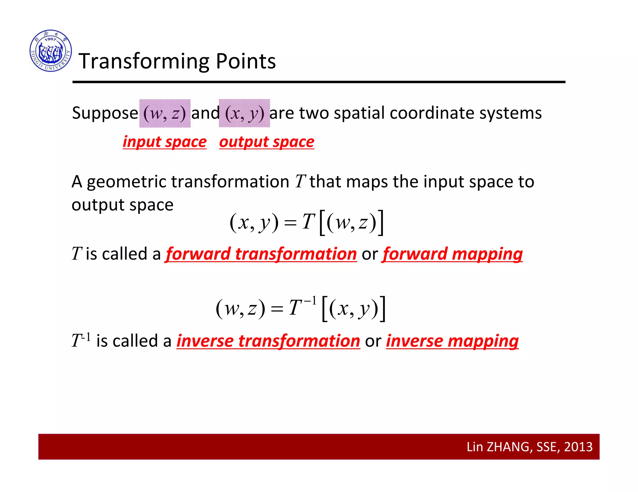
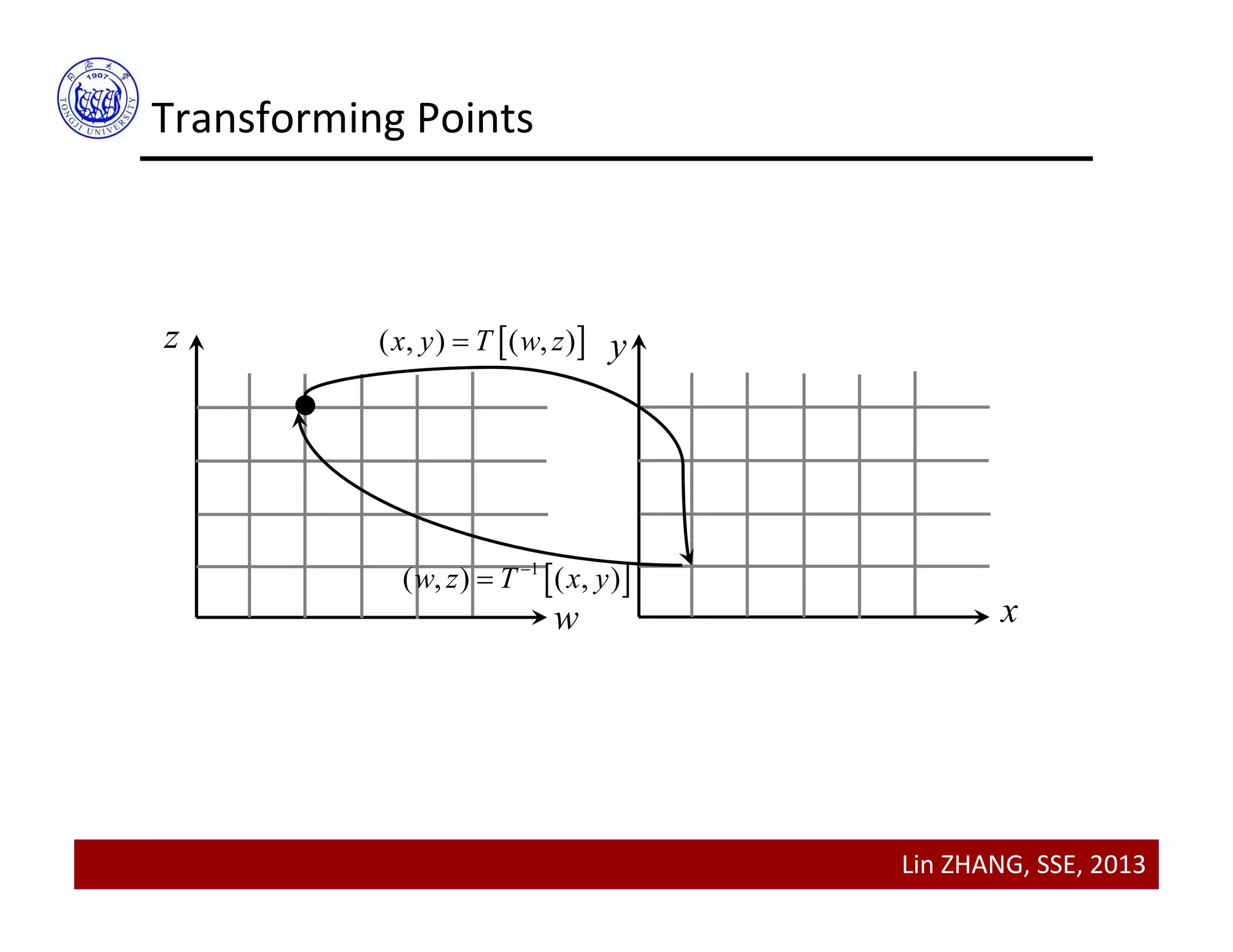
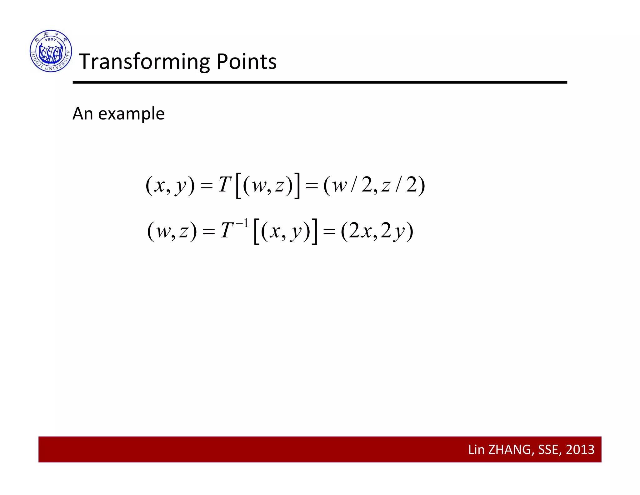
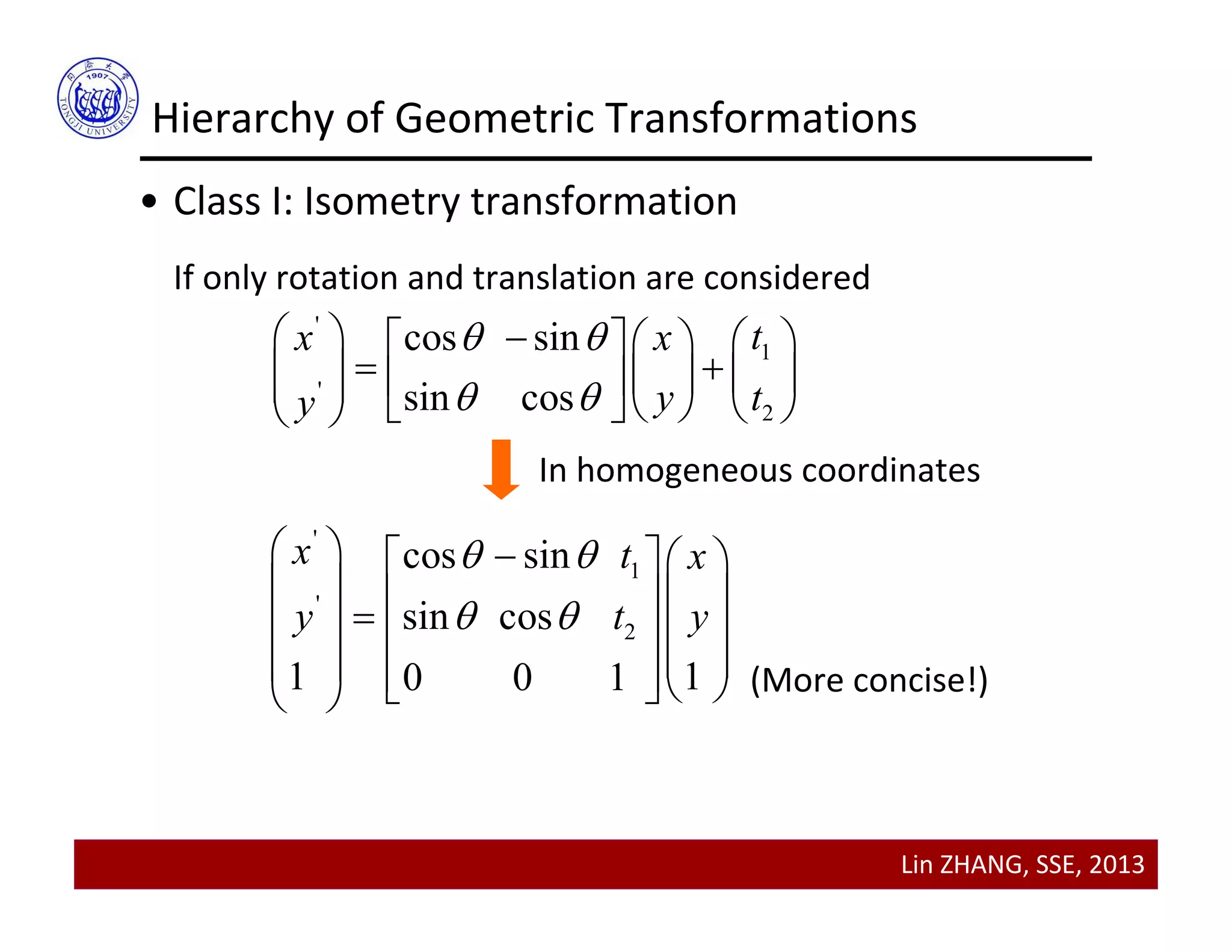
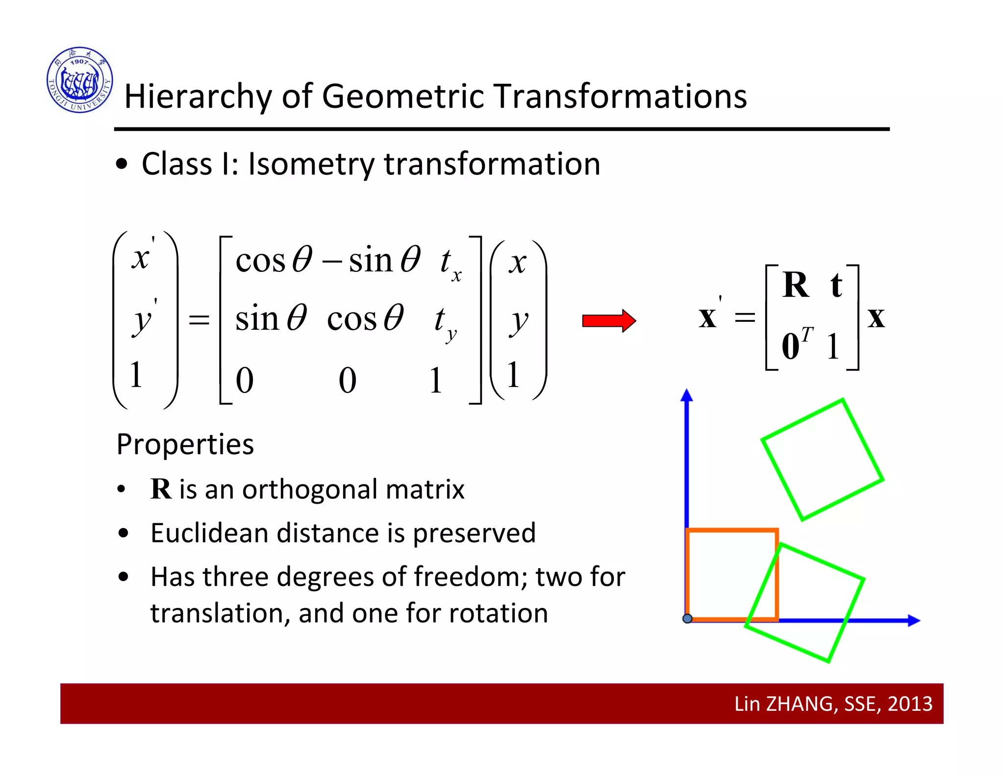
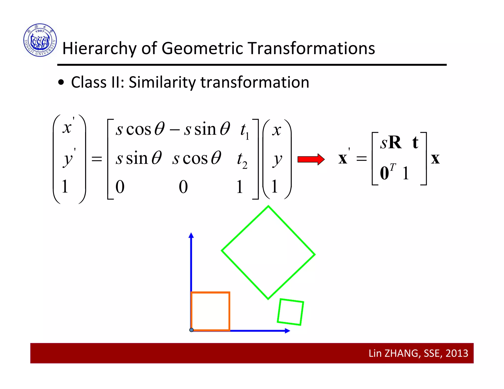
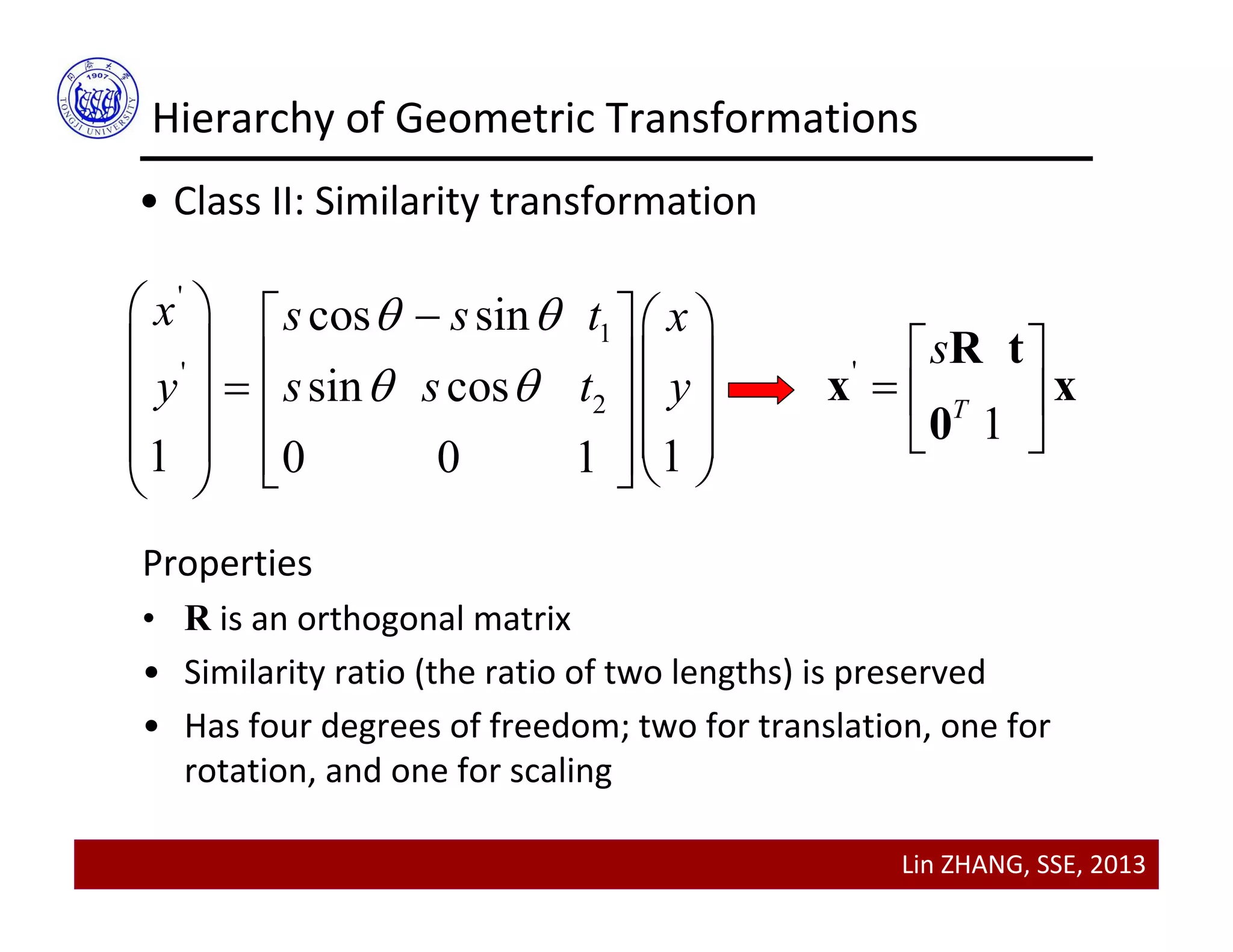
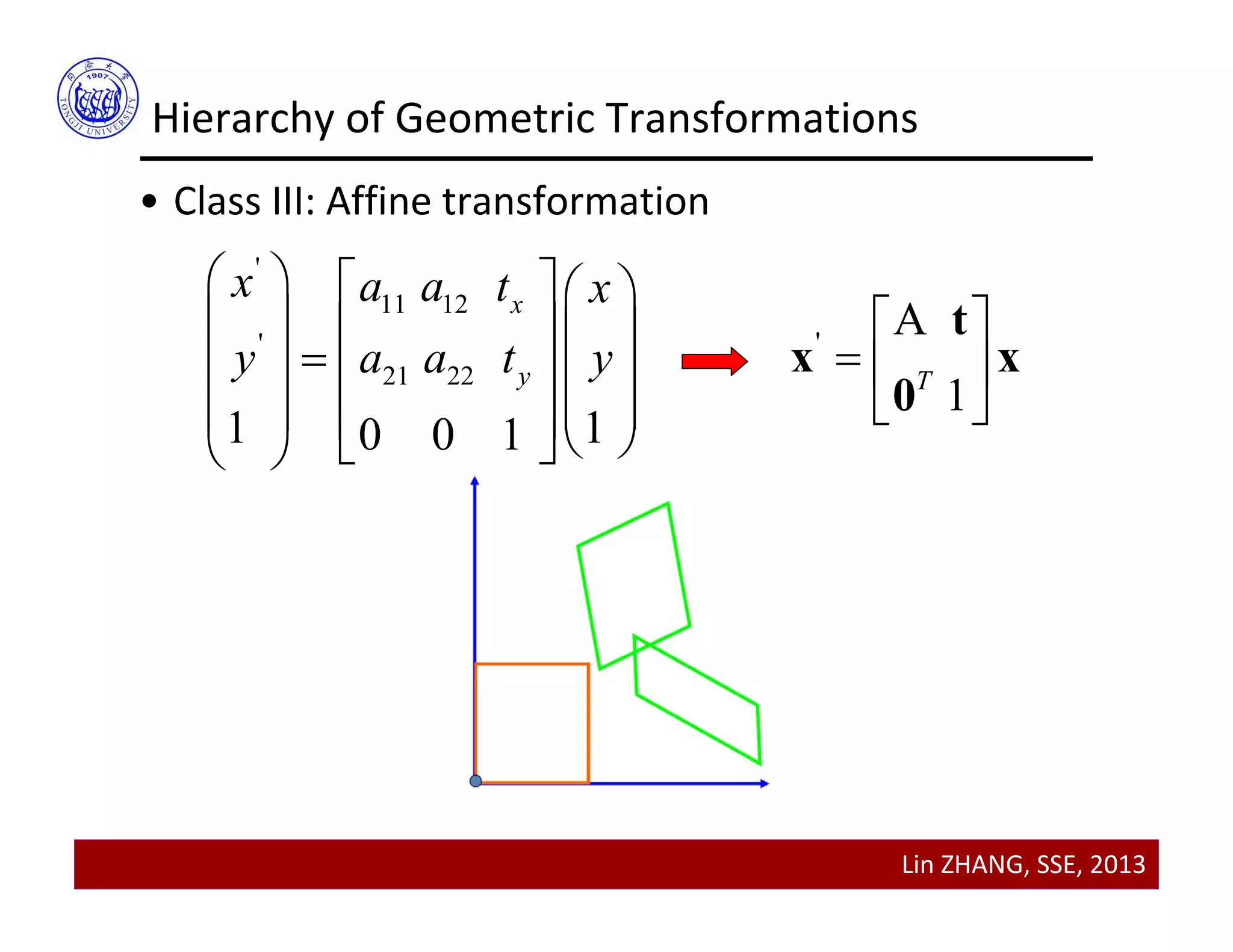
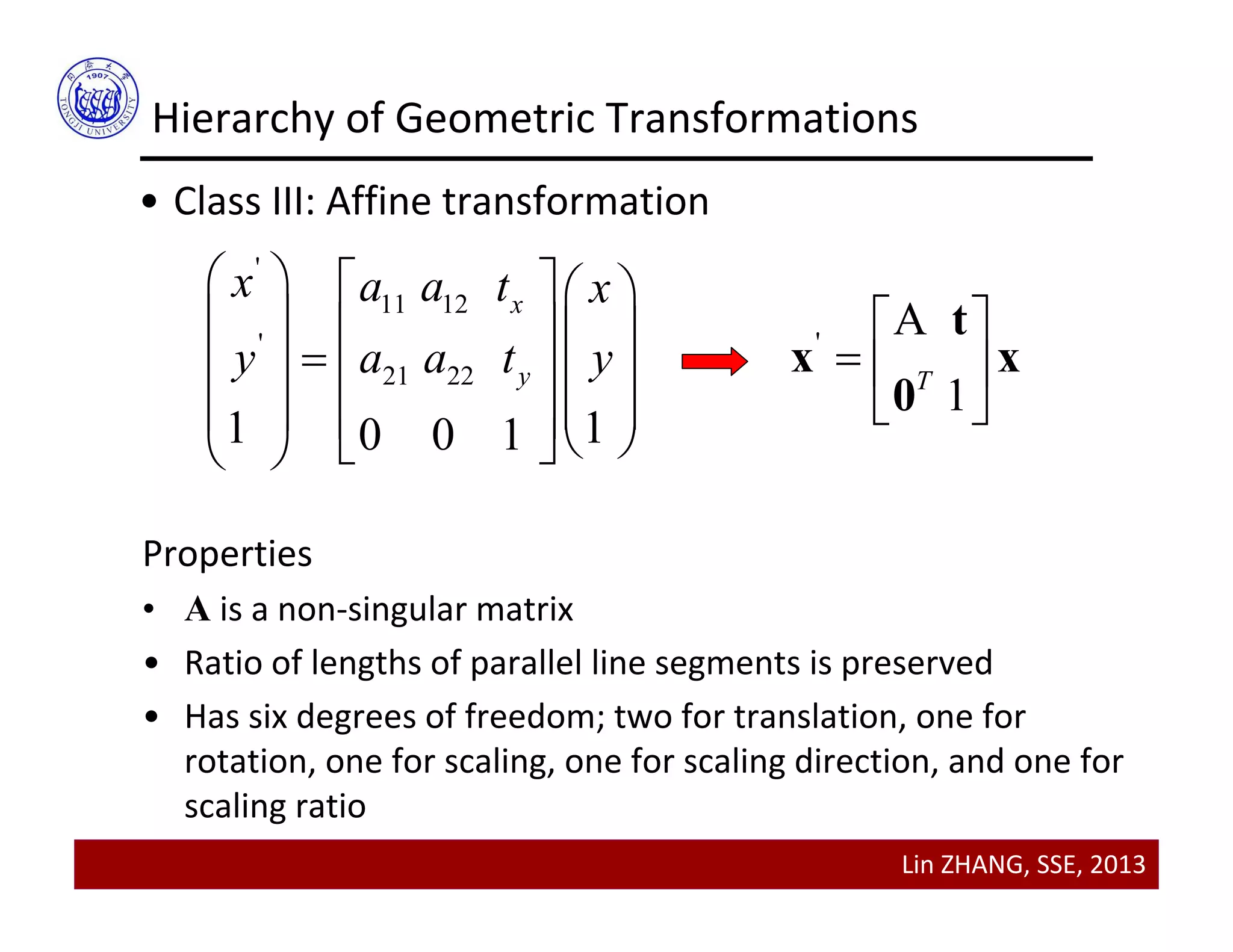
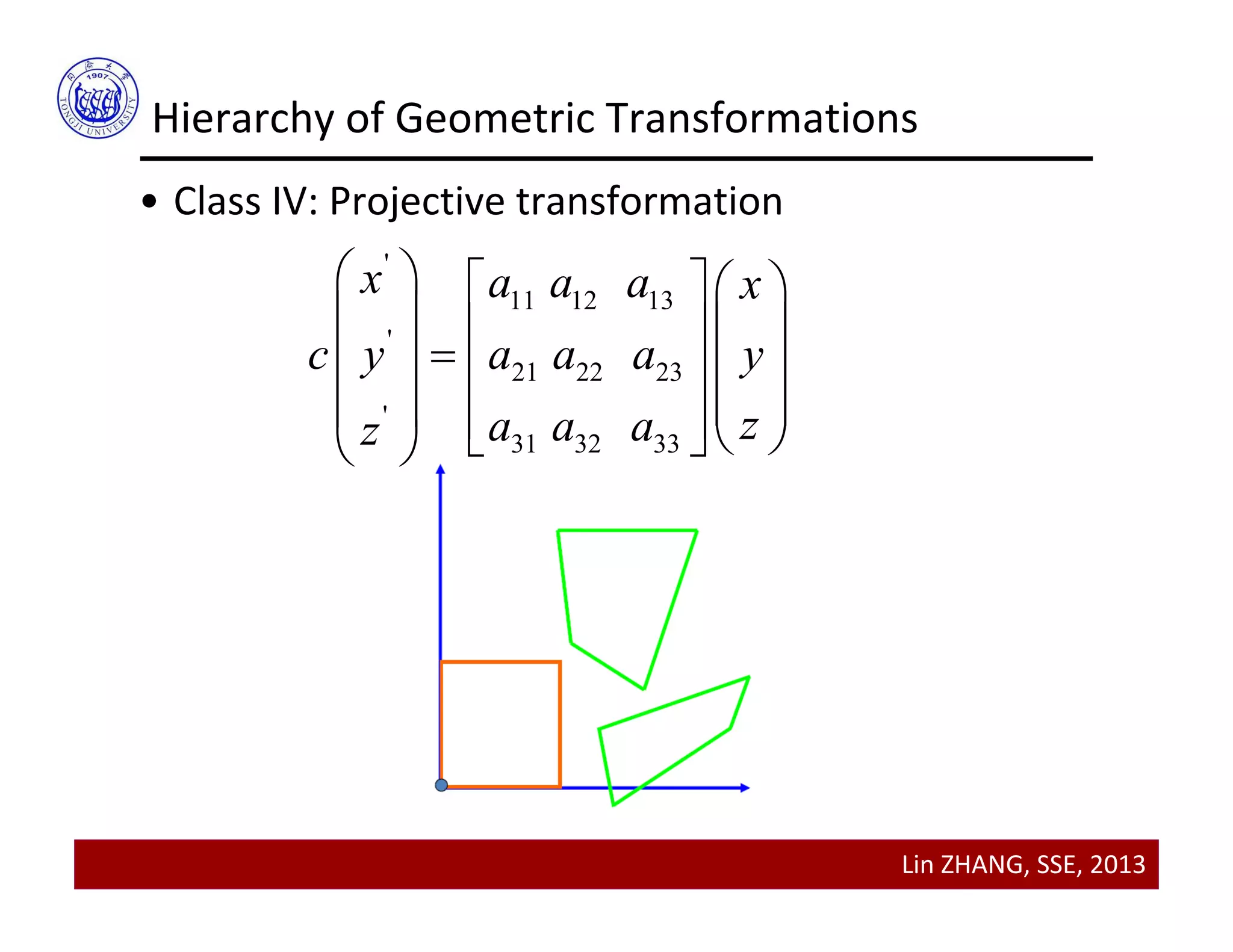
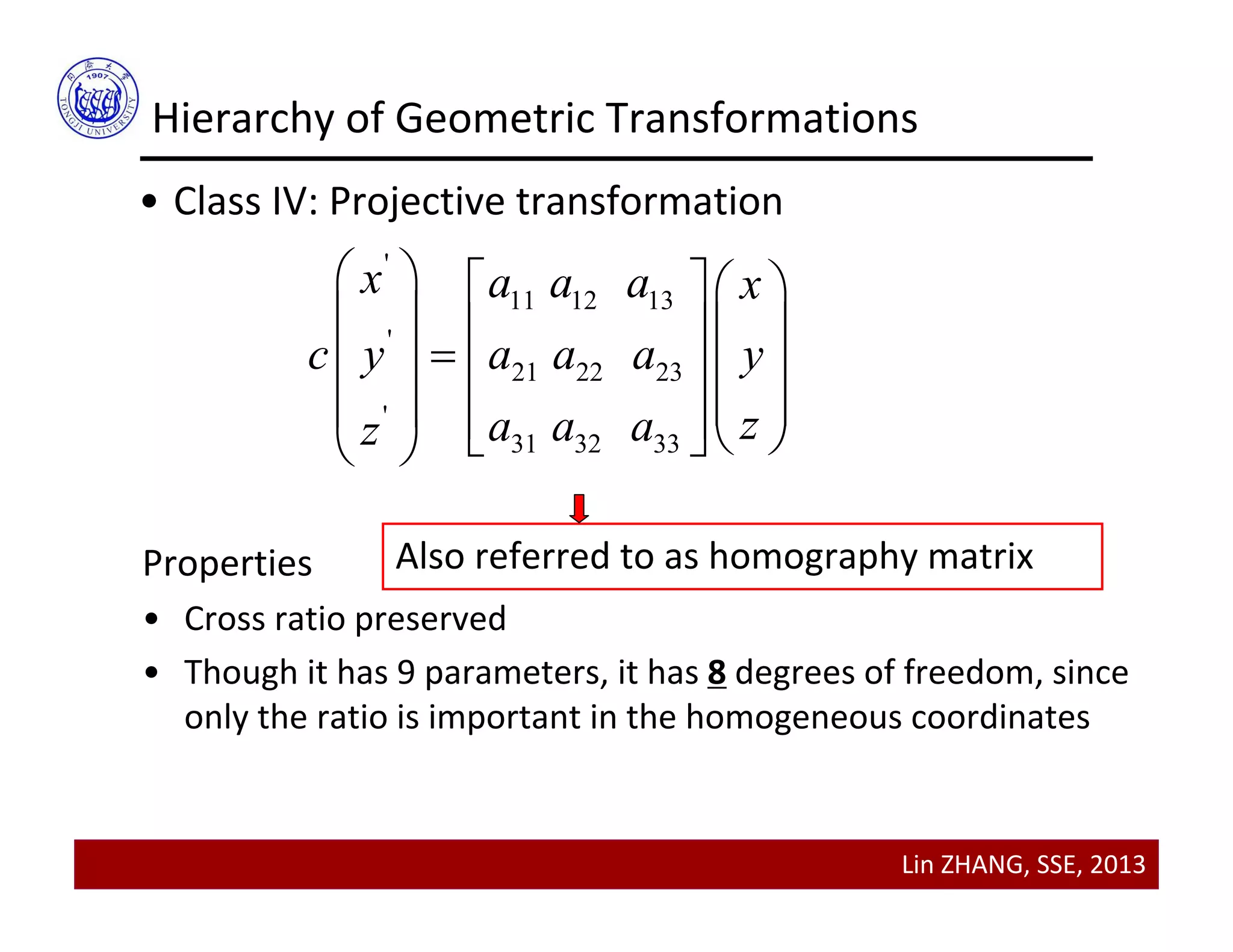
This document discusses geometric transformations and image registration. It begins by explaining how geometric transformations modify the spatial relationship between pixels in an image. It then covers transforming points using forward and inverse transformations. The rest of the document describes a hierarchy of geometric transformations including isometries, similarities, affine transformations, and projective transformations. It explains how to apply these transformations to images using interpolation and provides MATLAB examples. The document concludes by discussing image registration.
![Lin ZHANG, SSE, 2013
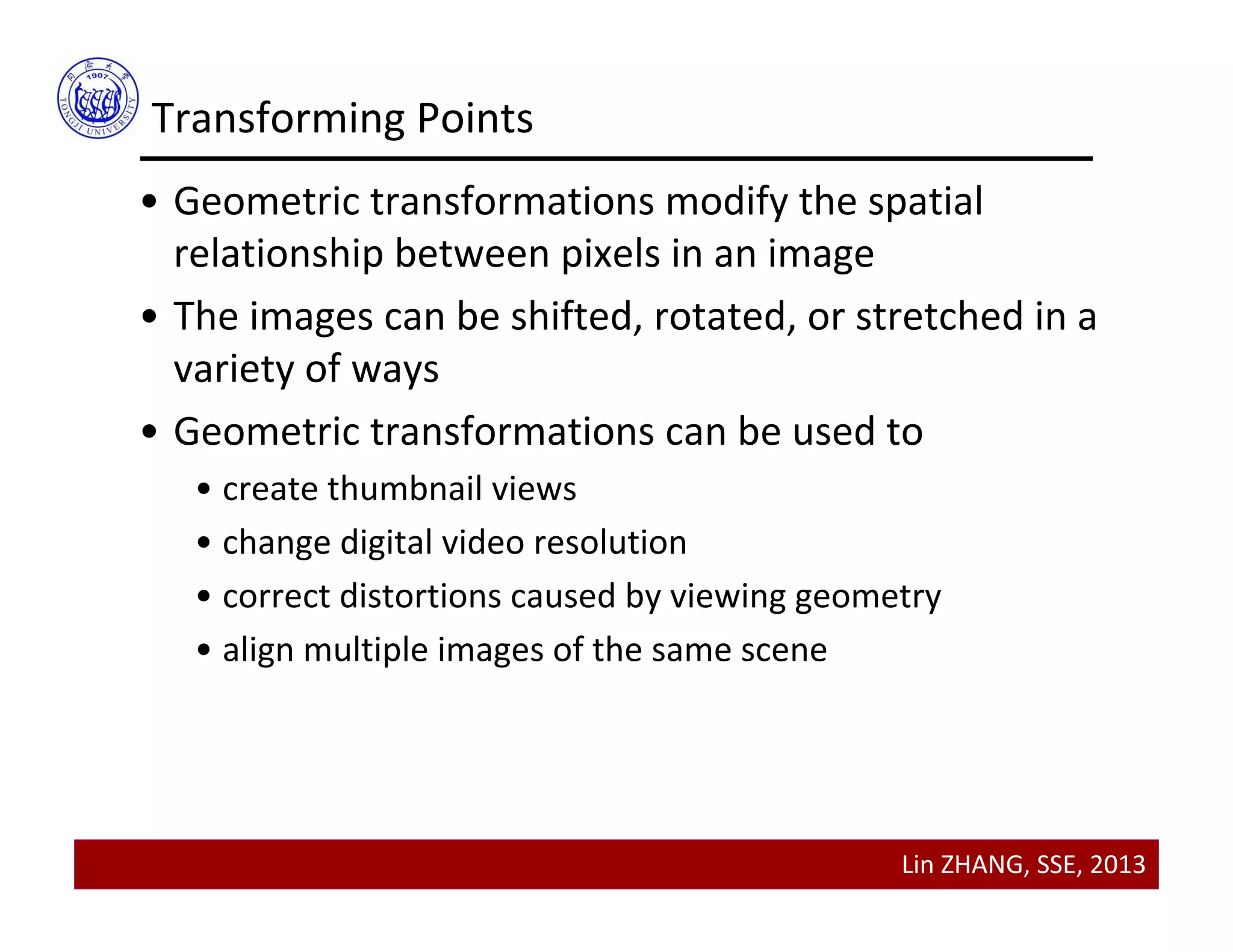
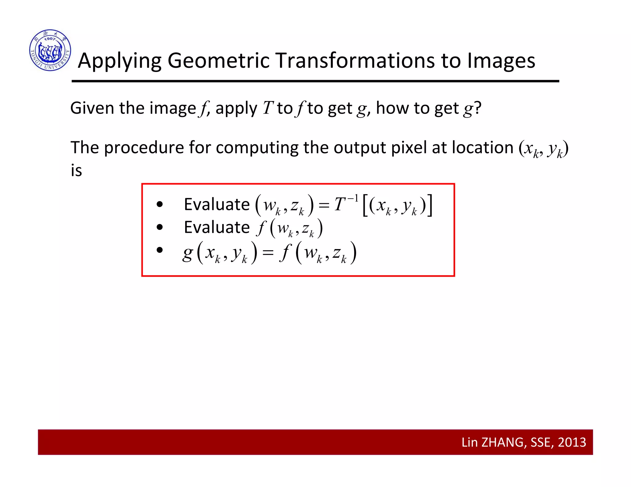
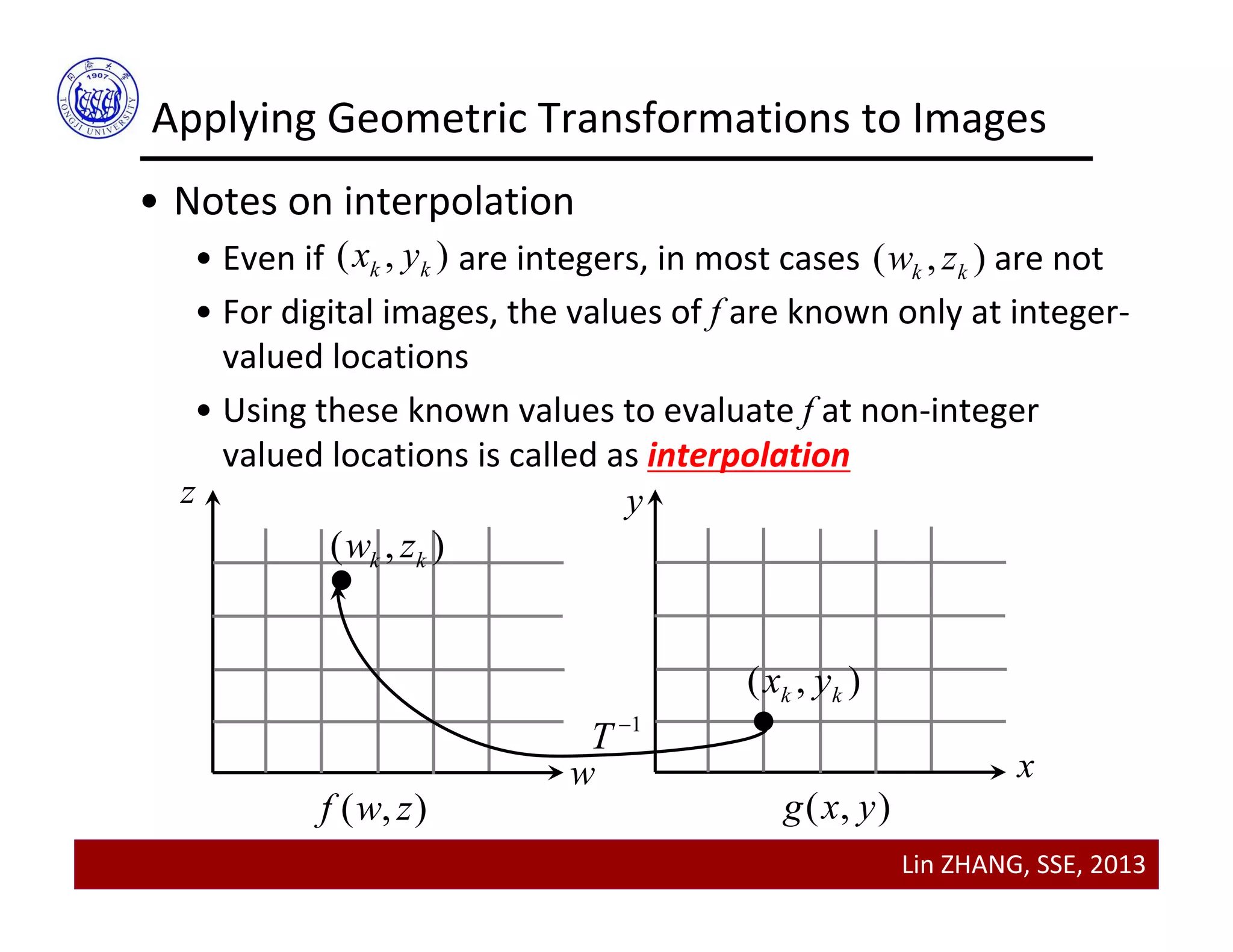
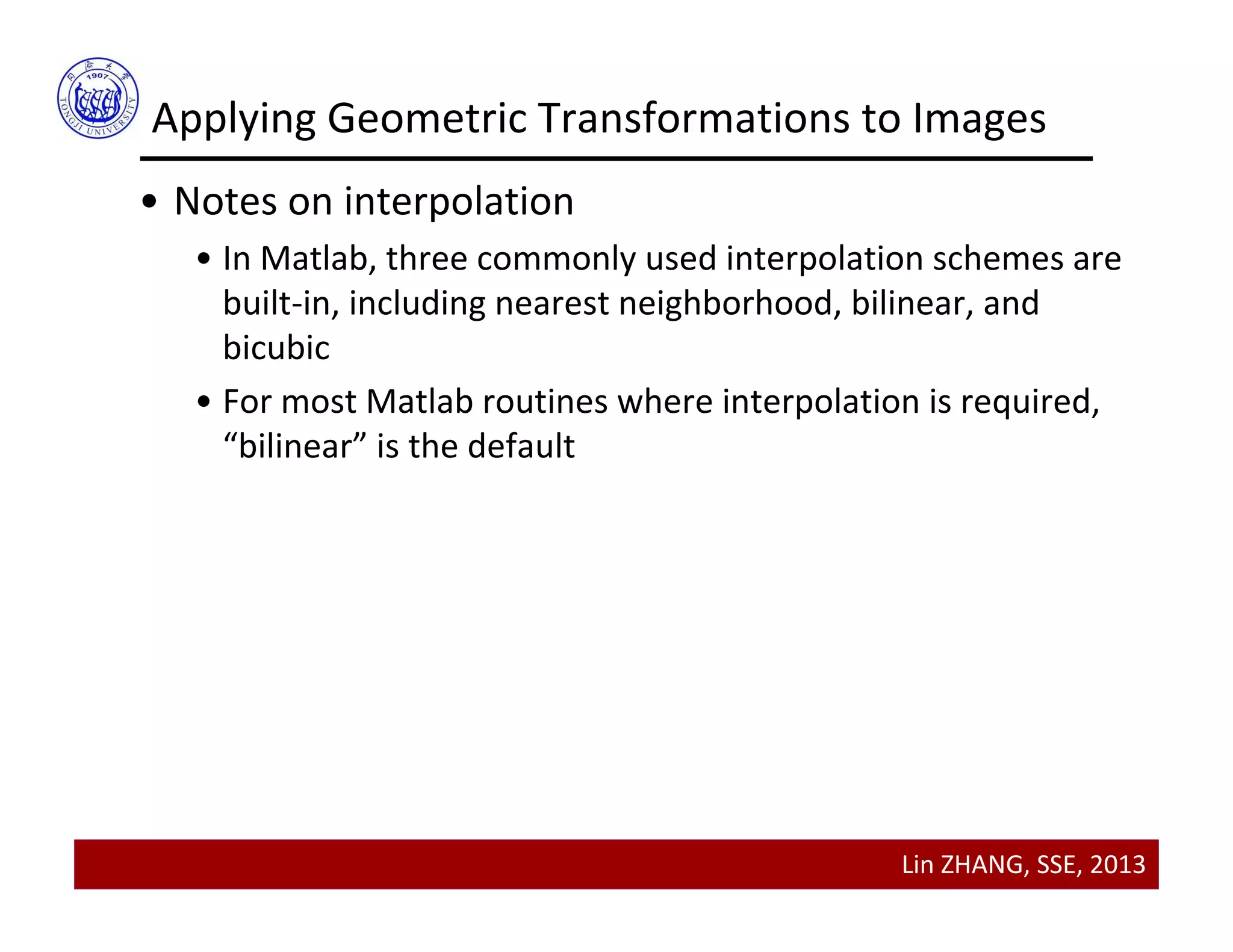
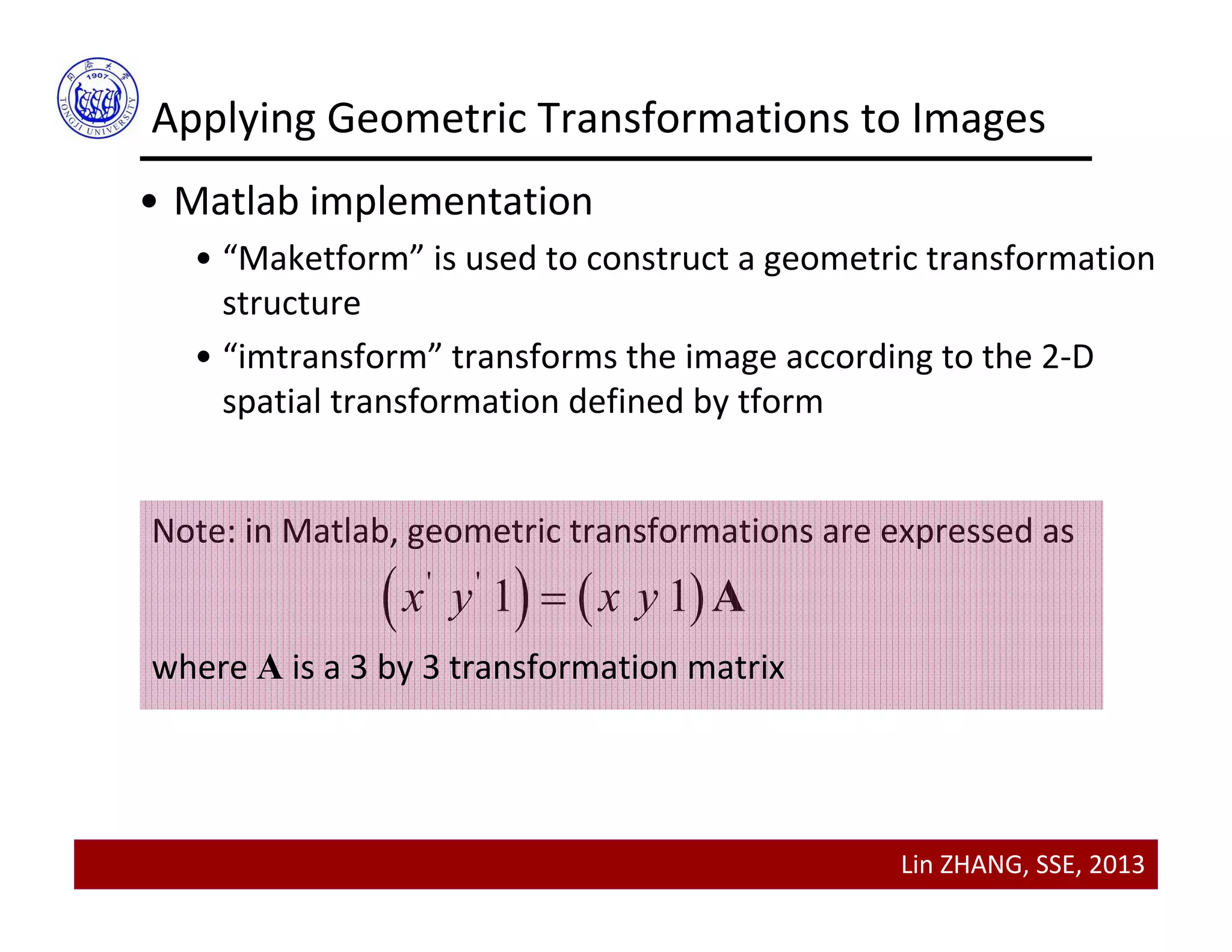
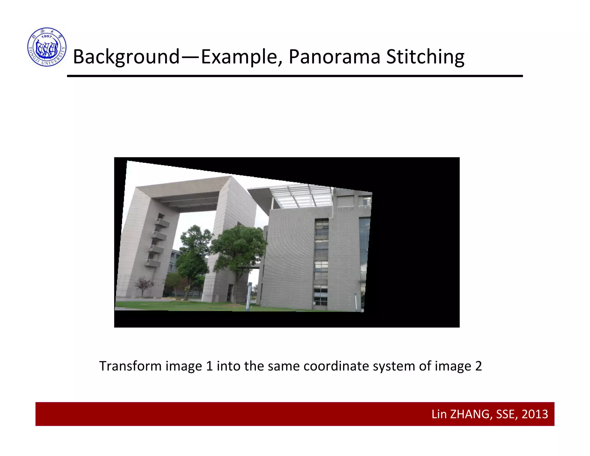
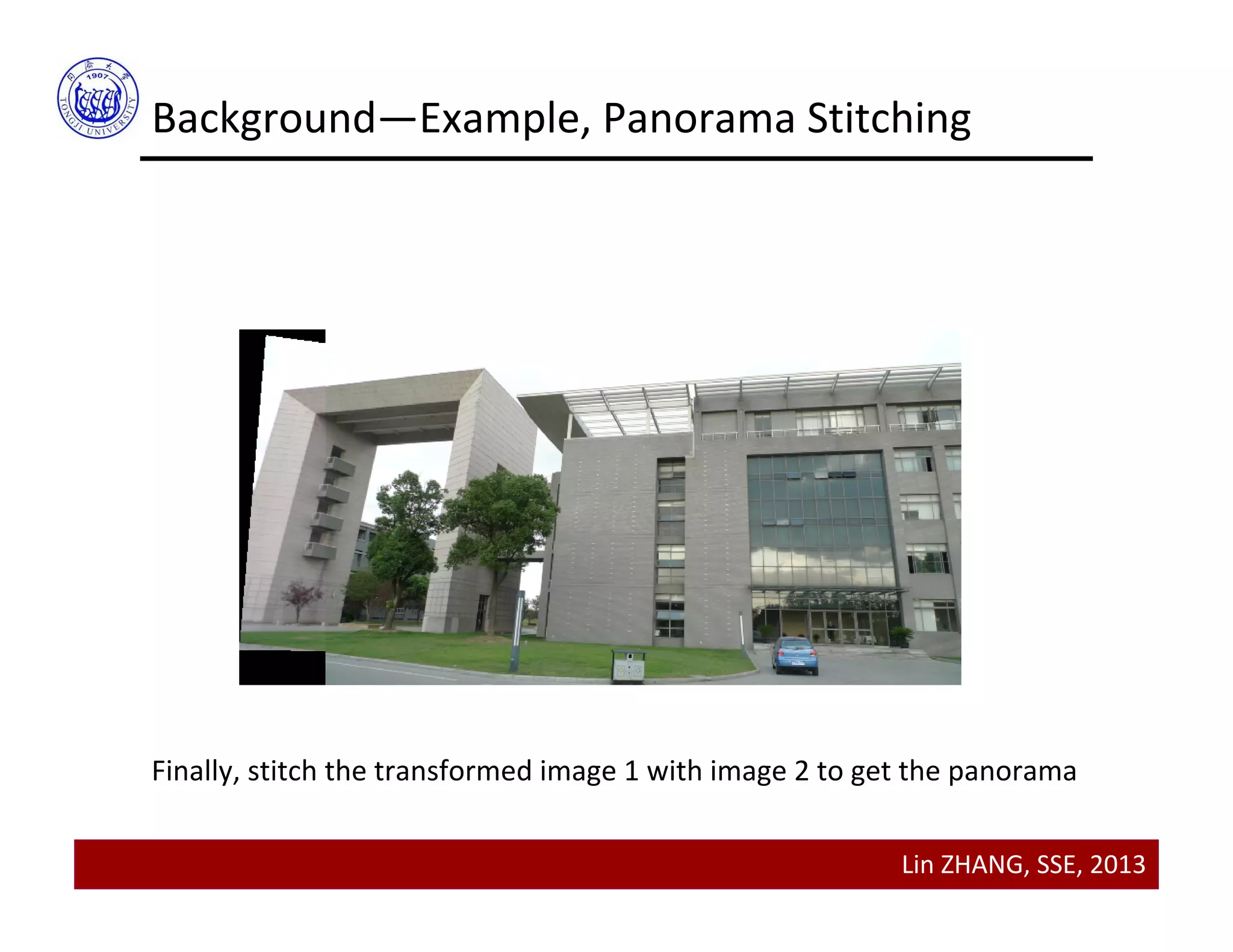
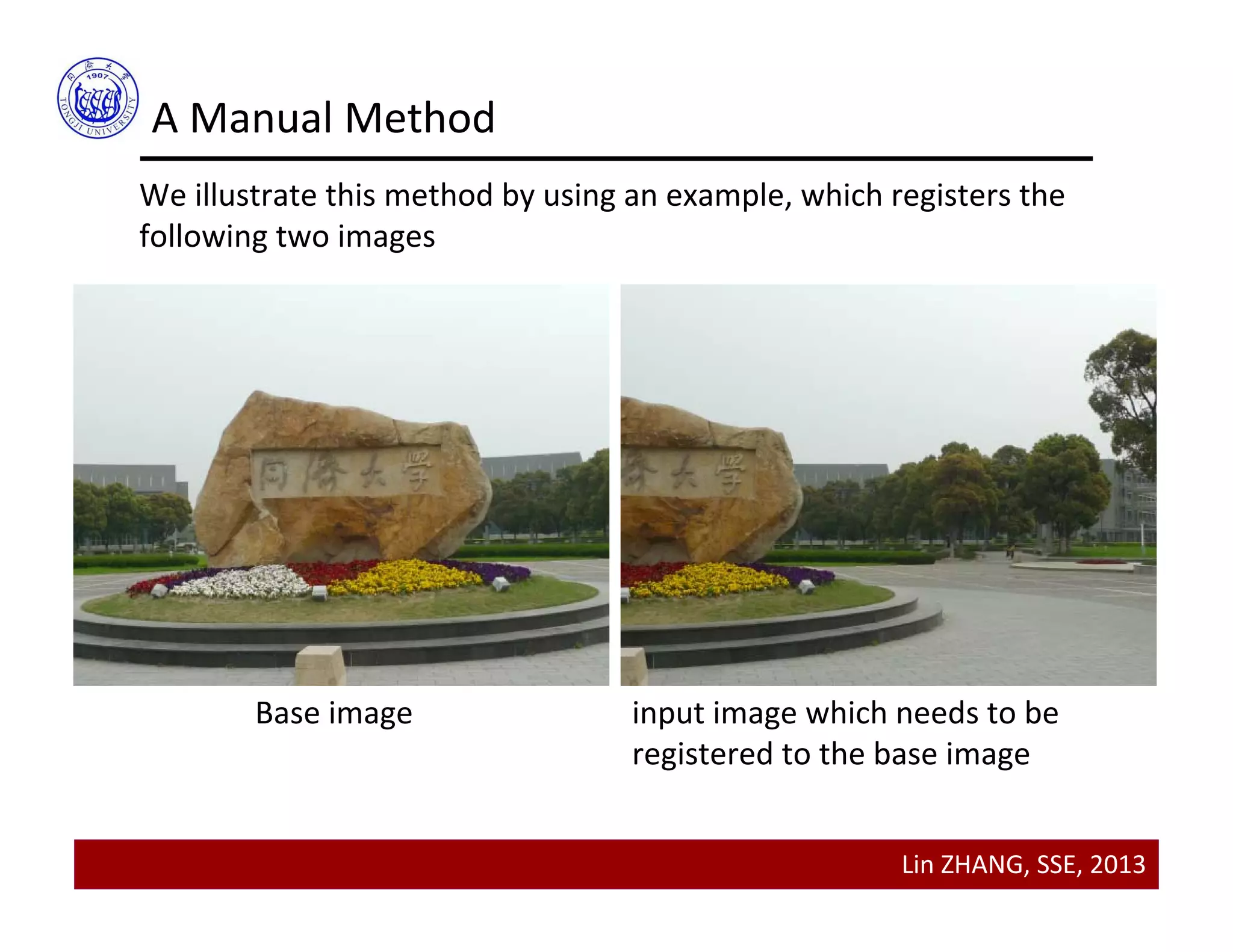
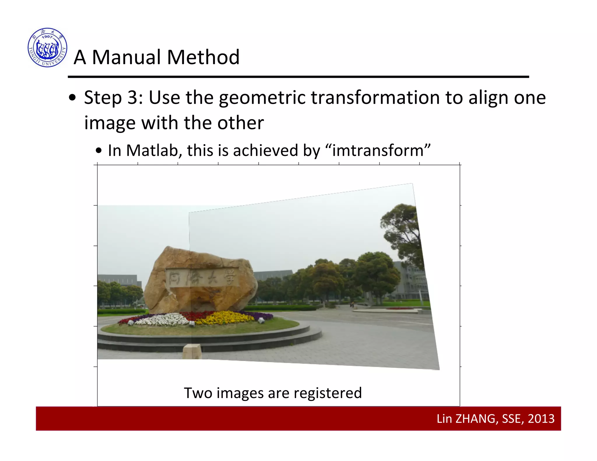
Applying Geometric Transformations to Images
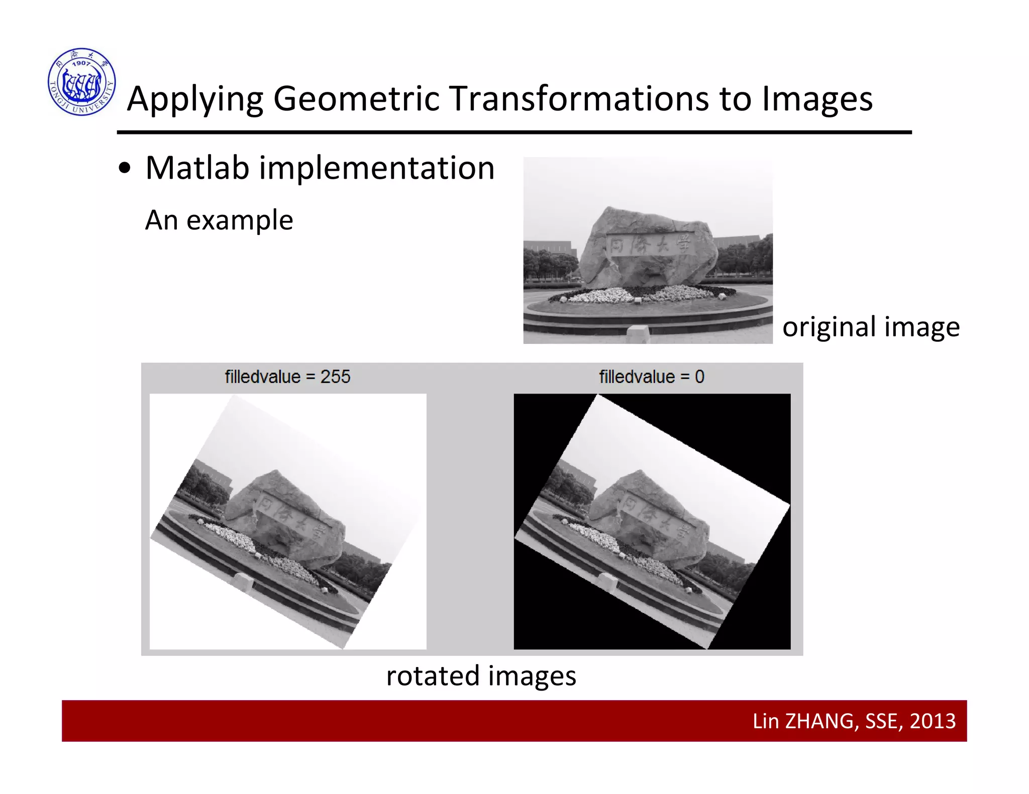
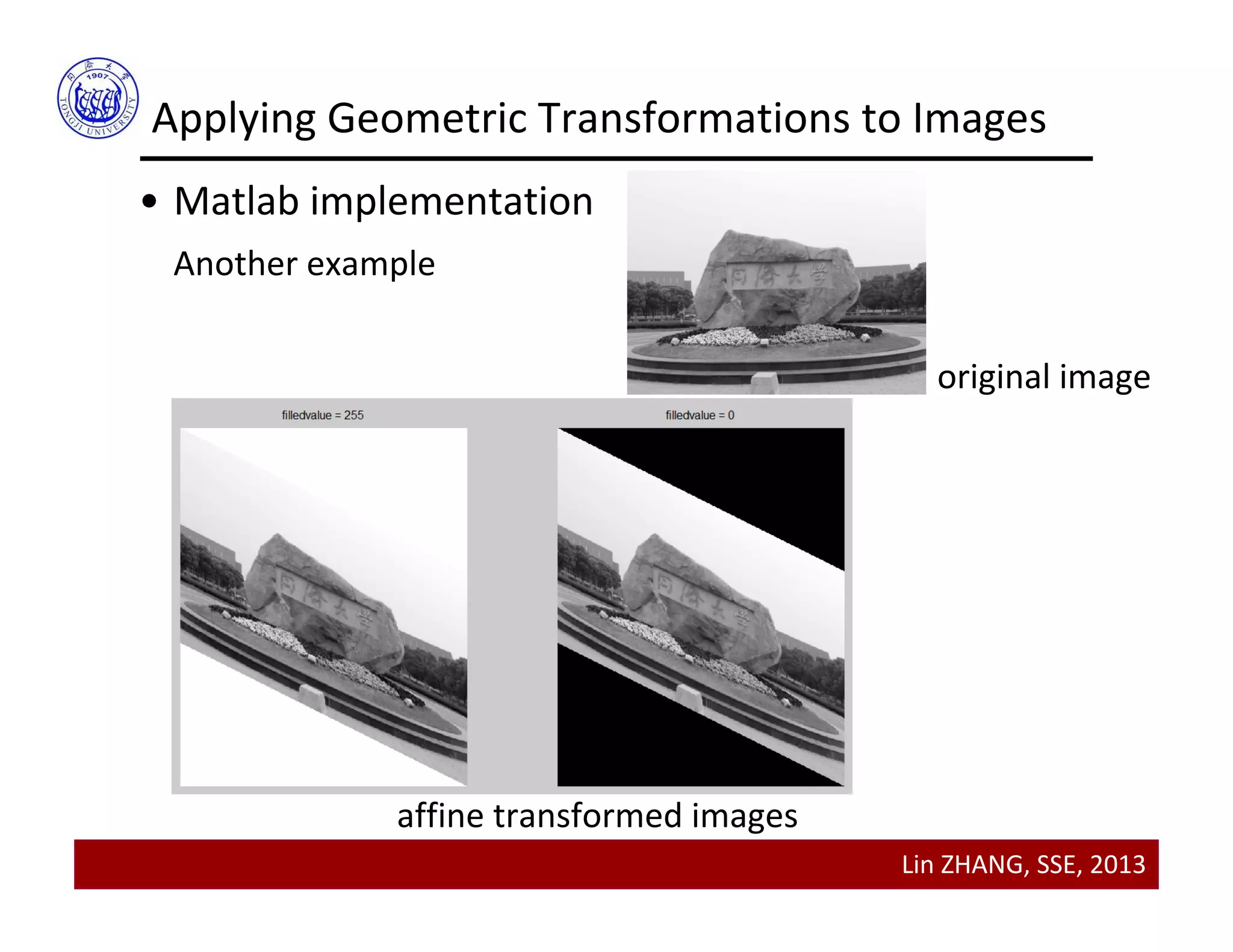
• Matlab implementation
An example
im = imread('tongji.bmp');
theta = pi/6;
rotationMatrix = [cos(theta) sin(theta) 0;-sin(theta) cos(theta) 0;0 0 1];
tformRotation = maketform('affine',rotationMatrix);
rotatedIm = imtransform(im, tformRotation,'FillValues',255);
figure;
subplot(1,2,1); imshow(rotatedIm,[]);
rotatedIm = imtransform(im, tformRotation,'FillValues',0);
subplot(1,2,2); imshow(rotatedIm,[]);](https://image.slidesharecdn.com/lecture06-geometrictransformationsandimageregistration-150420215326-conversion-gate01/75/Lecture-06-geometric-transformations-and-image-registration-21-2048.jpg)
![Lin ZHANG, SSE, 2013
Applying Geometric Transformations to Images
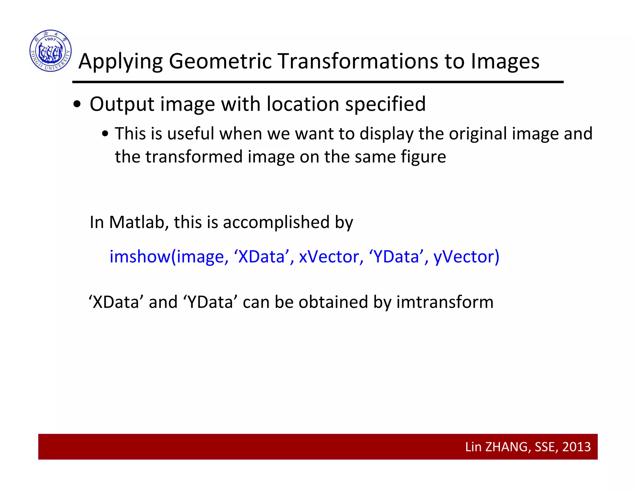
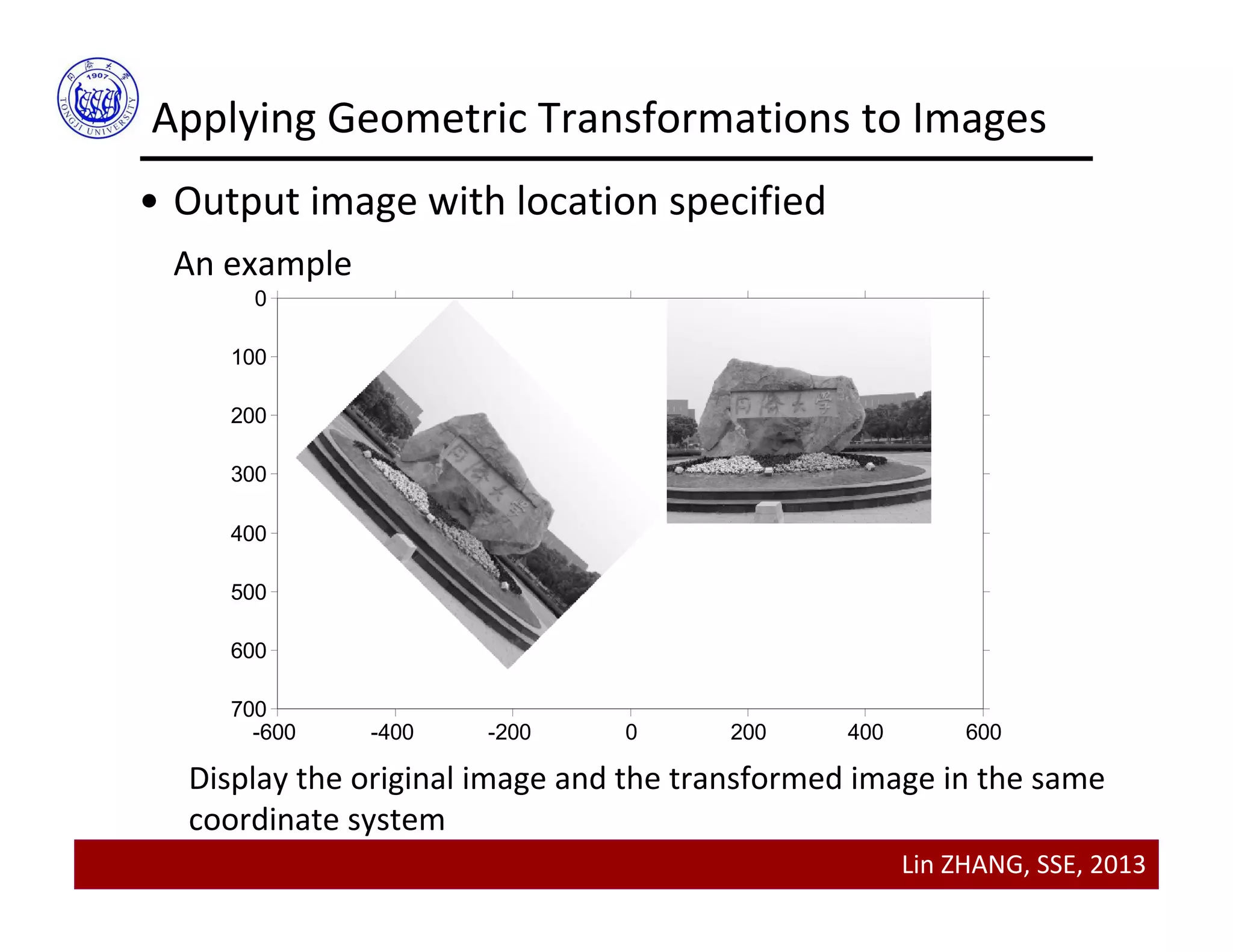
• Output image with location specified
An example
im = imread('tongji.bmp');
theta = pi/4;
affineMatrix = [cos(theta) sin(theta) 0;-sin(theta) cos(theta) 0;-300 0 1];
tformAffine = maketform('affine',affineMatrix);
[affineIm, XData, YData] = imtransform(im, tformAffine,'FillValues',255);
figure; imshow(im,[]);
hold on
imshow(affineIm,[],'XData',XData,'YData',YData);
axis auto
axis on](https://image.slidesharecdn.com/lecture06-geometrictransformationsandimageregistration-150420215326-conversion-gate01/75/Lecture-06-geometric-transformations-and-image-registration-25-2048.jpg)


![[DSC Europe 25] Dobrica Cosic - From Electrons to Innovation: How Granular Da...](https://cdn.slidesharecdn.com/ss_thumbnails/h4qk69zereaumbceubgr-dobrica-cosic-from-electrons-to-innovation-how-granular-data-and-analytics-are--251218085301-b982fb14-thumbnail.jpg?width=640&height=640&fit=bounds)


![[DSC Europe 25] Jean Del Rosario - How to Reduce GenAI Costs up to 73.45%.pptx](https://cdn.slidesharecdn.com/ss_thumbnails/zjehcwqsiwjisav1znml-5-251217093201-eae4440a-thumbnail.jpg?width=640&height=640&fit=bounds)
![[DSC Europe 25] Francisco Prado Moreno - Model Validation in the Age of AI: T...](https://cdn.slidesharecdn.com/ss_thumbnails/2igqvkir1yd2yzlhoylg-3-251215095918-6676c4e6-thumbnail.jpg?width=640&height=640&fit=bounds)

![[DSC Europe 25] Ivan Peric - Intelligence Swarm Logic and Techno-Functional M...](https://cdn.slidesharecdn.com/ss_thumbnails/7my7c97fsduiccadgavw-2-251212103249-5a03f7c6-thumbnail.jpg?width=640&height=640&fit=bounds)
![[DSC Europe 25] Hans Kleinsman - The Compliance Gearbox: How Tax Tech Mediate...](https://cdn.slidesharecdn.com/ss_thumbnails/dxdytie1toel0hr90bjs-2-251212103250-174fdbe7-thumbnail.jpg?width=640&height=640&fit=bounds)


![[DSC Europe 25] Debmalya Biswas - Agentification: the art of transforming man...](https://cdn.slidesharecdn.com/ss_thumbnails/r5azlggvtqiaiiusrqdr-4-251212103249-5a12c89b-thumbnail.jpg?width=640&height=640&fit=bounds)
![[DSC Europe 25] Branko Urosevic -Rethinking Financial Talent: Integrating Cod...](https://cdn.slidesharecdn.com/ss_thumbnails/8jjrus8ttko6qj64f58f-3-251212103250-642c6374-thumbnail.jpg?width=640&height=640&fit=bounds)
![[DSC Europe 25] Behzad Hosseini - AI Agents in the Wild: Deploying Models tha...](https://cdn.slidesharecdn.com/ss_thumbnails/3qtejajvsjqrzwfept2c-10-251212103250-7f2b1068-thumbnail.jpg?width=640&height=640&fit=bounds)