Download as PDF, PPTX


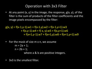


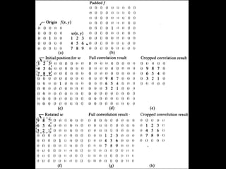


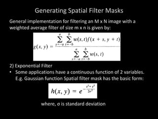


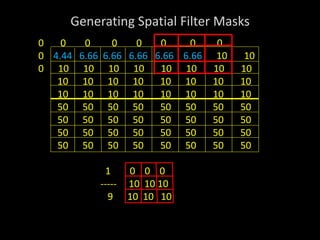

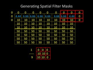


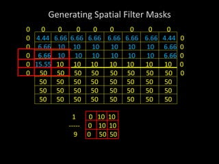
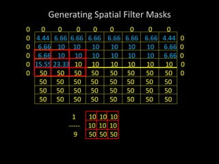


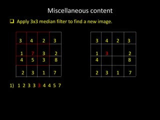
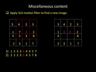


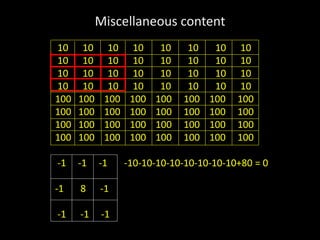


1) The document discusses spatial filtering of digital images, which refers to modifying images by applying filters in the spatial domain rather than the frequency domain. 2) Spatial filters are applied by using a kernel or mask over an image to perform operations on pixels within the mask's area. Common operations include averaging, edge detection, and noise removal. 3) A 3x3 mask is demonstrated as the simplest case, where the response value for the center pixel is the sum of the pixel values multiplied by the corresponding mask weights. This allows various filters to be generated for different purposes.


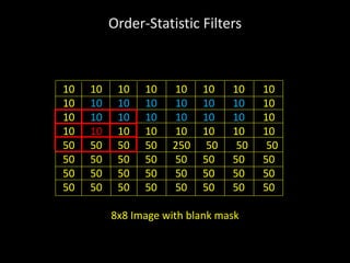
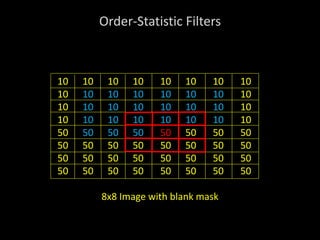
![Lec5_AIP [Spatial Filtering] (1).pptxt767686777](https://cdn.slidesharecdn.com/ss_thumbnails/lec5aipspatialfiltering1-240729201851-b222fde6-thumbnail.jpg?width=640&height=640&fit=bounds)