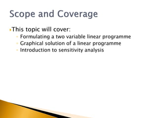
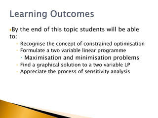
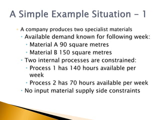
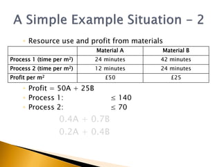
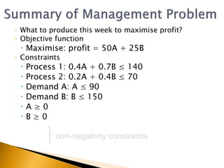
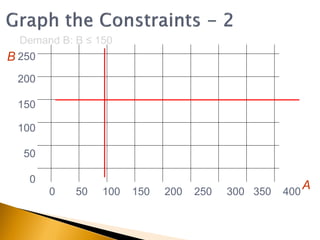
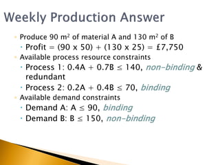
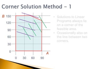
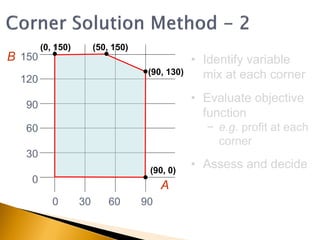
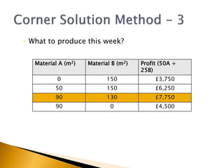
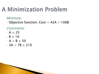
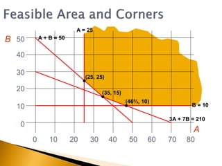
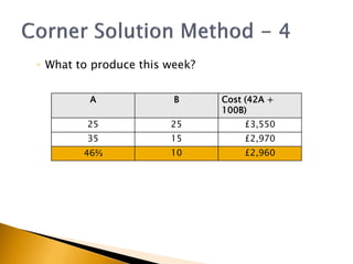
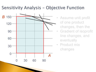
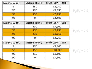
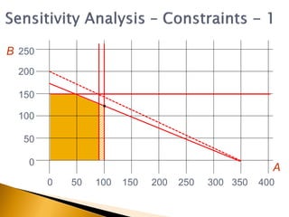
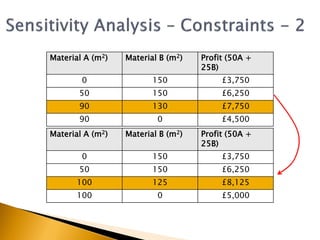
The document covers linear programming, focusing on formulating two-variable programs and graphical solutions while introducing sensitivity analysis. It demonstrates practical applications through scenarios involving resource constraints and maximizing profit from two specialist materials. By the end, students should be able to recognize constrained optimization, formulate problems, and appreciate sensitivity analysis.

1. Topic10:
Linear Programming

2. This topic will cover:
◦ Formulating a two variable linear programme
◦ Graphical solution of a linear programme
◦ Introduction to sensitivity analysis

3. By the end of this topic students will be able
to:
◦ Recognise the concept of constrained optimisation
◦ Formulate a two variable linear programme
 Maximisation and minimisation problems
◦ Find a graphical solution to a two variable LP
◦ Appreciate the process of sensitivity analysis

4. ◦ A company produces two specialist materials
 Available demand known for following week:
 Material A 90 square metres
 Material B 150 square metres
 Two internal processes are constrained:
 Process 1 has 140 hours available per
week
 Process 2 has 70 hours available per week
 No input material supply side constraints

5. ◦ Resource use and profit from materials
◦ Profit = 50A + 25B
◦ Process 1: ≤ 140
◦ Process 2: ≤ 70
Material A Material B
Process 1 (time per m2) 24 minutes 42 minutes
Process 2 (time per m2) 12 minutes 24 minutes
Profit per m2 £50 £25
0.4A + 0.7B
0.2A + 0.4B

6. ◦ What to produce this week to maximise profit?
◦ Objective function
 Maximise: profit = 50A + 25B
◦ Constraints
 Process 1: 0.4A + 0.7B ≤ 140
 Process 2: 0.2A + 0.4B ≤ 70
 Demand A: A ≤ 90
 Demand B: B ≤ 150
 A ≥ 0
 B ≥ 0
non-negativity constraints

7. 0 50 100 150 200 250 300 350 400
250
200
150
100
50
0
A
B
Demand A: A ≤ 90

8. 0 50 100 150 200 250 300 350 400
250
200
150
100
50
0
A
B
Demand B: B ≤ 150

9. 0 50 100 150 200 250 300 350 400
250
200
150
100
50
0
A
B
Process 1: 0.4A + 0.7B ≤ 140

10. 0 50 100 150 200 250 300 350 400
250
200
150
100
50
0
A
B
Process 2: 0.2A + 0.4B ≤ 70

11. 0 50 100 150 200 250 300 350 400
250
200
150
100
50
0
A
B
The Feasible Area

12. 0 30 60 90
150
120
90
60
30
0
A
B
The Feasible Area • Graph the objective
function
• Profit = 50A + 25B
• Profit =
£3,000
• Profit =
£5,250
• Profit =
£6,750
• Profit =
£7,750

13. ◦ Produce 90 m2 of material A and 130 m2 of B
 Profit = (90 x 50) + (130 x 25) = £7,750
◦ Available process resource constraints
 Process 1: 0.4A + 0.7B ≤ 140, non-binding &
redundant
 Process 2: 0.2A + 0.4B ≤ 70, binding
◦ Available demand constraints
 Demand A: A ≤ 90, binding
 Demand B: B ≤ 150, non-binding

14. 0 30 60 90
150
120
90
60
30
0
A
B • Solutions to Linear
Programs always lie
on a corner of the
feasible area.
• Occasionally also on
the line between two
corners.

15. 0 30 60 90
150
120
90
60
30
0
A
B • Identify variable
mix at each corner
• Evaluate objective
function
− e.g. profit at each
corner
• Assess and decide(90, 0)
(90, 130)
(50, 150)(0, 150)

16. ◦ What to produce this week?
Material A (m2) Material B (m2) Profit (50A +
25B)
0 150 £3,750
50 150 £6,250
90 130 £7,750
90 0 £4,500

17. Minimize:
◦ Objective function: Cost = 42A + 100B
Constraints
◦ A ≥ 25
◦ B ≥ 10
◦ A + B ≥ 50
◦ 3A + 7B ≥ 210

18. 0 10 20 30 40 50 60 70 80
50
40
30
20
10
0
A
B
A = 25
B = 10
A + B = 50
3A + 7B = 210
(25, 25)
(46⅔, 10)
(35, 15)

19. ◦ What to produce this week?
A B Cost (42A +
100B)
25 25 £3,550
35 15 £2,970
46⅔ 10 £2,960

20. 0 30 60 90
150
120
90
60
30
0
A
B • Assume unit profit
of one product
changes, then the
• Gradient of isoprofit
line changes, and
eventually
• Product mix
changes

21. Material A (m2) Material B (m2) Profit (50A + 25B)
0 150 £3,750
50 150 £6,250
90 130 £7,750
90 0 £4,500
Material A (m2) Material B (m2) Profit (25A + 50B)
0 150 £7,500
50 150 £8,750
90 130 £8,750
90 0 £2,250
Material A (m2) Material B (m2) Profit (20A + 60B)
0 150 £9,000
50 150 £10,000
90 130 £9,600
90 0 £1,800
PB:PA = 0.5
PB:PA = 2.0
PB:PA = 3.0

22. 0 50 100 150 200 250 300 350 400
250
200
150
100
50
0
A
B

23. Material A (m2) Material B (m2) Profit (50A +
25B)
0 150 £3,750
50 150 £6,250
90 130 £7,750
90 0 £4,500
Material A (m2) Material B (m2) Profit (50A +
25B)
0 150 £3,750
50 150 £6,250
100 125 £8,125
100 0 £5,000

24. 0 50 100 150 200 250 300 350 400
250
200
150
100
50
0
A
B

25. 0 50 100 150 200 250 300 350 400
250
200
150
100
50
0
A
B

26. By the end of this topic students will be able
to:
◦ Recognise the concept of constrained optimization
◦ Formulate a two variable linear programme
 Maximisation and minimisation problems
◦ Find a graphical solution to a two variable LP
◦ Appreciate the process of sensitivity analysis

27. ◦ Hillier, F. and Lieberman. G. Introduction to
Operations Research. McGraw Hill
◦ Keast, S. and Towler M. Rational Decision-Making
for Managers. Wiley.
◦ Wisniewski, M. Quantitative Methods for Decision
Makers. FT Prentice Hall.

28. Any Questions?