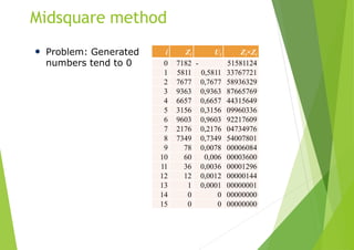
This presentation discusses methods for generating pseudo-random numbers and testing their randomness. It introduces the midsquare method as the first arithmetic generator but notes its tendency to generate numbers that approach zero. The linear congruential method and combined linear congruential generators are presented as improved approaches. Statistical tests for randomness like the Kolmogorov-Smirnov test and chi-square test are also summarized to evaluate the uniformity and independence of generated random numbers.

1. Presentation on Pseudo Random-Number
Generation

2. Contents
• Pseudo-Random Numbers and their properties
• Generating Random Numbers
• Midsquare Method
• Linear Congruential Method
• Combined Linear Congruential Method
• Tests for Random Numbers

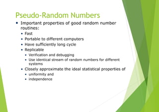
3. Pseudo-Random Numbers
• Approach: Arithmetically generation
(calculation) of random numbers
• “Pseudo”, because generating numbers using a
known method removes the potential for true
randomness.
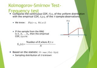
• Goal: To produce a sequence of numbers in
[0,1] that simulates, or imitates, the ideal
properties of random numbers (RN).

4. Pseudo-Random Numbers
• Important properties of good random number
routines:
• Fast
• Portable to different computers
• Have sufficiently long cycle
• Replicable
• Verification and debugging
• Use identical stream of random numbers for different
systems
• Closely approximate the ideal statistical properties of
• uniformity and
• independence

5. Pseudo-Random Numbers:
Properties
• Two important statistical properties:
• Uniformity
• Independence
• Random number Ri must be independently drawn from a
uniform distribution with PDF:
1
22
1
x2
0
1
0
E(R)  xdx  
0 1
PDF for random numbers
f(x)
x
1, 0  x 1
f(x)= 0. otherwise

6. Generation of Random Numbers
• Midsquare method
• Linear Congruential Method (LCM)
• Combined Linear Congruential Generators (CLCG)
• Random-Number Streams

7. Midsquare method
• First arithmetic generator: Midsquare method
• von Neumann and Metropolis in 1940s
• The Midsquare method:
• Start with a four-digit positive integer Z0
• Compute: to obtain an integer with up to eight
digits
• Take the middle four digits for the next four-digit number
2
0 0 0Z  Z Z
i Zi Ui Zi×Zi
0 7182 - 51581124
1 5811 0.5811 33767721
2 7677 0.7677 58936329
3 9363 0.9363 87665769
…

8. Midsquare method
• Problem: Generated
numbers tend to 0
i Zi Ui Zi×Zi
0 7182 - 51581124
1 5811 0,5811 33767721
2 7677 0,7677 58936329
3 9363 0,9363 87665769
4 6657 0,6657 44315649
5 3156 0,3156 09960336
6 9603 0,9603 92217609
7 2176 0,2176 04734976
8 7349 0,7349 54007801
9 78 0,0078 00006084
10 60 0,006 00003600
11 36 0,0036 00001296
12 12 0,0012 00000144
13 1 0,0001 00000001
14 0 0 00000000
15 0 0 00000000

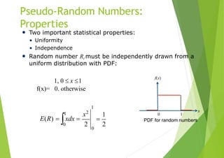
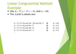
9. Linear Congruential Method
• To produce a sequence of integers X1, X2, … between 0 and
m-1 by following a recursive relationship:
Xi1  (aXi  c)mod m, i  0,1,2,...
• Assumption: m > 0 and a < m, c < m, X0 < m
• The selection of the values for a, c, m, and X0 drastically
affects the statistical properties and the cycle length
• The random integers Xi are being generated in [0, m-1]
The multiplier The increment The modulus

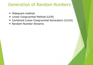
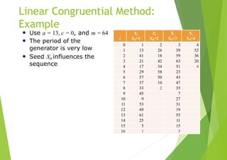
10. Linear Congruential Method
• Convert the integers Xi to random numbers
• Note:
• Xi  {0, 1, ...,m-1}
• Ri  [0,(m-1)/m]
, i 1,2,...R 
m
Xi
i

11. Linear Congruential Method:
Example
• Use X0 = 27, a = 17, c = 43, and m =100.
• The Xi and Ri values are:
X1 = (17×27+43) mod 100 = 502 mod 100 =2 Æ R1 = 0.02
X2 = (17×2 +43) mod 100 = 77 Æ R2 = 0.77
X3 = (17×77+43) mod 100 = 52 Æ R3 = 0.52
X4 = (17×52+43) mod 100 = 27
…
Æ R3 = 0.27

12. Linear Congruential Method:
Example
• Use a = 13, c = 0, and m = 64
• The period of the
generator is very low
• Seed X0 influences the
sequence
i
Xi
X0=1
Xi
X0=2
Xi
X0=3
Xi
X0=4
0 1 2 3 4
1 13 26 39 52
2 41 18 59 36
3 21 42 63 20
4 17 34 51 4
5 29 58 23
6 57 50 43
7 37 10 47
8 33 2 35
9 45 7
10 9 27
11 53 31
12 49 19
13 61 55
14 25 11
15 5 15
16 1 3

13. General Congruential
Generators
• Linear Congruential Generators are a special case of
generators defined by:
Xi 1  g(Xi , Xi1,…) mod m
• where g() is a function of previous Xi’s
• Xi  [0, m-1], Ri = Xi /m
• Quadratic congruential generator
• Defined by: g( X , X )  aX 2
 bX  c
i i1 i i1
• Multiple recursive generators
• Defined by: g(Xi , Xi1,…)  a1 Xi  a2 Xi1  ak Xik
• Fibonacci generator
• Defined by: Xi1g(Xi , Xi1)  Xi

14. Combined Linear Congruential
Generators• Reason: Longer period generator is needed because of the
increasing complexity of simulated systems.
• Approach: Combine two or more multiplicative congruential
generators.
• Let Xi,1, Xi,2, …, Xi,k be the i-th output from k different
multiplicative congruential generators.
• The j-th generator X•,j:
• has prime modulus mj, multiplier aj, and period mj -1
• produces integers Xi,j approx ~ Uniform on [0, mj – 1]
• Wi,j = Xi,j - 1 is approx ~ Uniform on integers on [0, mj -2]
 cj ) mod mjXi1, j  (aj Xi

15. Tests for Random Numbers
• When to use these tests:
• If a well-known simulation language or random-number generator is
used, it is probably unnecessary to test
• If the generator is not explicitly known or documented, e.g.,
spreadsheet programs, symbolic/numerical calculators, tests should
be applied to many sample numbers.
• Types of tests:
• Theoretical tests: evaluate the choices of m, a, and c without actually
generating any numbers
• Empirical tests: applied to actual sequences of numbers produced.
• Our emphasis.

16. Kolmogorov-Smirnov Test-
Frequency test• Compares the continuous CDF, F(x), of the uniform distribution
with the empirical CDF, SN(x), of the N sample observations.
• We know:
• If the sample from the RNG
is R1, R2, …, RN, then the empirical
CDF, SN(x) is:
• Based on the statistic: D = max | F(x) - SN(x)|
• Sampling distribution of D is known
F(x)  x, 0  x 1
Number of Ri where Ri  x
NNS (x) 
0 1
F(x)
x

17. Kolmogorov-Smirnov Test
• The test consists of the
following steps
• Step 1: Rank the data from
smallest to largest
R(1) ≤ R(2) ≤ ... ≤ R(N)
• Step 2: Compute
• Step 3: Compute D = max(D+, D-)
• Step 4: Get D for the
significance level 
• Step 5: If D ≤ D accept,
otherwise reject H0
 N

i 1
D
 maxR 




N
D
 maxi
 R (i) 1iN
(i)
1iN

Kolmogorov-Smirnov Critical Values

18. Kolmogorov-Smirnov Test
6.18
i/N 0.20 0.40 0.60 0.80 1.00
i/N – R(i) 0.15 0.26 0.16 - 0.07
R(i) –(i-1)/N 0.05 - 0.04 0.21 0.13
Step 2:
Step 3:
Step 4:
D = max(D+, D-) = 0.26
For  = 0.05,
D = 0.565 > D = 0.26
Hence, H0 is not rejected.
i 1 2 3 4 5 Arrange R(i) from
R(i) 0.05 0.14 0.44 0.81 0.93
smallest to largest
• Example: Suppose N=5 numbers: 0.44, 0.81, 0.14, 0.05,0.93.
Step 1:
D+ = max{i/N –R(i)}
D - = max{R(i) -(i-1)/N}

19. Chi-square Test- Frequency tests
• Chi-square test uses the sample statistic:
• Approximately the chi-square distribution with n-1 degrees of
freedom
• For the uniform distribution, Ei, the expected number in each class
is:
• Valid only for large samples, e.g., N ≥ 50
i1
n
Ei
2
(O  E )2
i i
0  
n
iE 
N
, where N is the total number of observations
Ei is the expected # in the i-th class
Oi is the observed # in the i-th classn is the # of classes

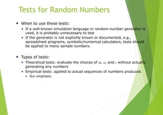
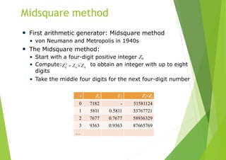
20. Chi-square Test:
Example
Interval Upper Limit Oi Ei Oi-Ei (Oi-Ei)^2 (Oi-Ei)^2/Ei
1 0.1 10 10 0 0 0
2 0.2 9 10 -1 1 0.1
3 0.3 5 10 -5 25 2.5
4 0.4 6 10 -4 16 1.6
5 0.5 16 10 6 36 3.6
6 0.6 13 10 3 9 0.9
7 0.7 10 10 0 0 0
8 0.8 7 10 -3 9 0.9
9 0.9 10 10 0 0 0
10 1.0 14 10 4 16 1.6
Sum 100 100 0 0 11.2
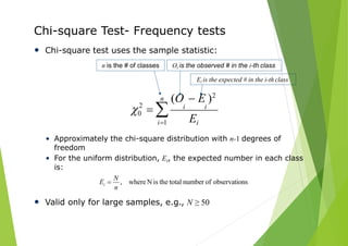
• Example with 100 numbers from [0,1], =0.05
• 10 intervals
0.05,9•  2 = 16.9
• Accept, since
0• X2 =11.2 <  2
0.05,9
0X2 =11.2
n
Eii1
2
(O  E)2
i i
0 