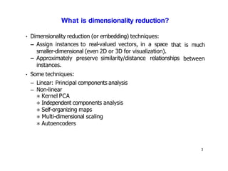
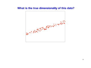
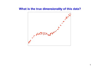
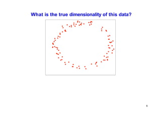
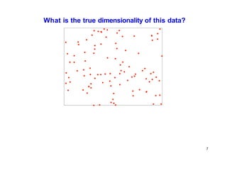
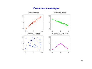
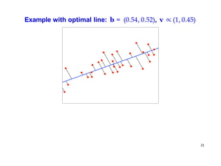
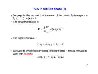
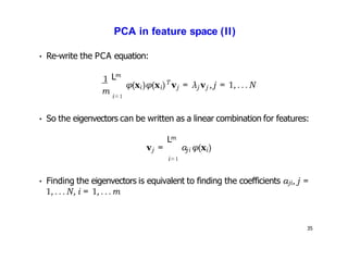
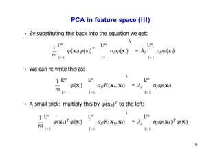
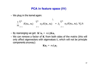
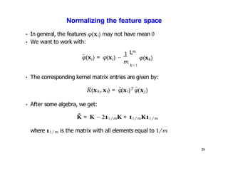
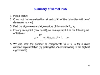
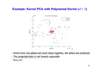
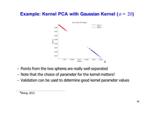
- Dimensionality reduction techniques assign instances to vectors in a lower-dimensional space while approximately preserving similarity relationships. Principal component analysis (PCA) is a common linear dimensionality reduction technique. - Kernel PCA performs PCA in a higher-dimensional feature space implicitly defined by a kernel function. This allows PCA to find nonlinear structure in data. Kernel PCA computes the principal components by finding the eigenvectors of the normalized kernel matrix. 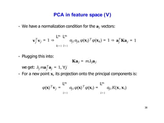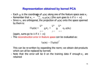- For a new data point, its representation in the lower-dimensional space is given by projecting it onto the principal components in feature space using the kernel trick, without explicitly computing features.

1. NEOTIA INSTITUTE OF TECHNOLOGY
MANAGEMENT AND SCIENCE
CONTINUOUS ASSESSMENT 1
MACHINE LEARNING
Name- Abdus Sadik Molla
Roll No. – 14400120004
Subject Name- Machine Learning
Subject Code – PEC-CS701E
Dep. – Computer Science and Engineering
Academic Session: 2023-24 (Odd Semester)

2. Dimensionality reduction. PCA. Kernel PCA.
• Dimensionality reduction
• Principal Component Analysis (PCA)
• Kernelizing PCA
• If we have time: Autoencoders
2

3. 3
What is dimensionality reduction?
• Dimensionality reduction (or embedding) techniques:
– Assign instances to real-valued vectors, in a space
smaller-dimensional (even 2D or 3D for visualization).
that is much
between
– Approximately preserve similarity/distance relationships
instances.
• Some techniques:
– Linear: Principal components analysis
– Non-linear
∗ Kernel PCA
∗ Independent components analysis
∗ Self-organizing maps
∗ Multi-dimensional scaling
∗ Autoencoders

4. What is the true dimensionality of this data?
4

5. What is the true dimensionality of this data?
5

6. What is the true dimensionality of this data?
6

7. What is the true dimensionality of this data?
7

8. 8
Remarks
• All dimensionality reduction techniques are based on an implicit
assumption that the data lies along some low-dimensional manifold
• This is the case for the first three examples, which lie along a 1-
dimensional manifold despite being plotted in 2D
• In the last example, the data has been generated randomly in 2D, so no
dimensionality reduction is possible without losing information
• The first three cases are in increasing order of difficulty, from the point
of view of existing techniques.

9. Simple Principal Component Analysis (PCA)
• Given: m instances, each being a length-n real vector.
• Suppose we want a 1-dimensional representation of that data, instead of
n-dimensional.
• Specifically, we will:
– Choose a line in Rn that “best represents” the data.
– Assign each data object to a point along that line.
?
?
?
?
9

10. 10
Reconstruction error
• Let the line be represented as b + αv for b, v ∈ Rn, α ∈R.
For convenience assume l v l = 1.
• Each instance xi is associated with a point on the line x̂i = b + αiv.
• We want to choose b, v, and the αi to minimize the total reconstruction
error over all data points, measured using Euclidean distance:
m
X
i=1
i i
R = lx − x̂ l 2

11. 11
A constrained optimization problem!
min
"'£m
i=1
lxi − (b + αiv)l2
w.r.t. b, v, αi, i = 1, .. .m
s.t. lvl2 = 1
• This is a quadratic objective with quadratic constraint
• Suppose we fix a v satisfying the condition, and find the best b and αi
given this v
• So, we solve:
minR = min
α,b
m
L
i=1
i i
lx − (b + α v)l 2
where R is the reconstruction error

12. 12
Solving the optimization problem (II)
• We write the gradient of R wrt to αi and set it to 0:
∂R
∂αi
2
i i i i
= 2lvl α − 2vx + 2bv = 0 ⇒ α = v ·(x − b)
where we take into account that lvl2 = 1.
• We write the gradient of R wrt b and set it to 0:
∇bR = 2mb − 2
i=1 i=1
xi + 2
m m
L L
αi v = 0
!
(1)
m
• From above:
L
i=1
m
L
αi = vT (xi − b) = vT
i=1
m
L
i=1
xi − mb
!
(2)

13. 13
Solving the optimization problem (III)
• By plugging (2) into (1) we get:
vT
m
L
i=1
xi − mb v =
m
L
i=1
xi − mb
• This is satisfied when:
m
L
i
x − mb = 0 ⇒ b =
1
m
i=1 i=1
m
L
xi
• This means that the line goes through the mean of the data
• By substituting αi, we get: x̂i = b + (vT (xi − b))v
• This means that instances are projected orthogonally on the line to get
the associated point.

14. Example data
14

15. Example with v ∝(1, 0.3)
15

16. 16
Finding the direction of the line
• Substituting αi = vT (xi − b) into our optimization problem we obtain a
new optimization problem:
maxv
"'£m
i=1
vT (xi − b)(xi − b)T v
s.t. lvl2 = 1
• The Lagrangian is:
L(v, λ) =
m
L
i=1
i i
T T
v (x − b)(x − b) v + λ − λl vl 2
• Let S =
"'£m
i=1
(xi − b)(xi − b)T be an n-by-n matrix, which we will call
the scatter matrix
• The solution to the problem, obtained by setting ∇vL = 0, is: Sv = λv.

17. 17
Optimal choice of v
• Recall: an eigenvector u of a matrix A satisfies Au = λu, where λ ∈ R
is the eigenvalue.
• Fact: the scatter matrix, S, has n non-negative eigenvaluesand n
orthogonal eigenvectors.
• The equation obtained for v tells us that it should be an eigenvector of
S.
• The v that maximizes vT Sv is the eigenvector of S with the largest
eigenvalue

18. 18
What is the scatter matrix
• S is an n × n matrix with
m
S(k, l) =
L
i=1
• Hence, S(k, l) is proportional to the estimated covariance between the
kth and lth dimension in the data.
(xi(k) − b(k))(xi(l) − b(l))

19. 19
Recall: Covariance
• Covariance quantifies a linear relationship (if any) between two random
variables X and Y.
1
Cov(X, Y) = E{(X − E(X))(Y − E(Y ))}
• Given m samples of X and Y, covariance can be estimated as
m
m
L
i=1
(xi − µX )(yi − µY ) ,
X
where µ = (1/m)
"'£m
i=1
xi and µY = (1/m)
"'£m
i=1 yi.
• Note: Cov(X, X) = Var(X).

20. Covariance example
0 5
Cov=−0.12338
10
0
5
10
Cov=7.6022 Cov=−3.8196
0 5 10
0
5
10
0 5 10
0
5
10
0
20
5 10
0
5
10
Cov=0.00016383

21. Example with optimal line: b = (0.54, 0.52), v ∝(1, 0.45)
21

22. 22
Remarks
• The line b + αv is the first principal component.
• The variance of the data along the line b + αv is as large as along any
other line.
• b, v, and the αi can be computed easily in polynomial time.

23. 23
Reduction to d dimensions
• More generally, we can create a d-dimensional representation of our data
by projecting the instances onto a hyperplane b + α1v1 + ... + αdvd.
• If we assume the vj are of unit length and orthogonal, then the optimal
choices are:
– b is the mean of the data (as before)
– The vj are orthogonal eigenvectors of S corresponding to its d largest
eigenvalues.
– Each instance is projected orthogonally on the hyperplane.

24. Remarks
• b, the eigenvalues, the vj, and the projections of the instances can all
be computing in polynomial time.
• The magnitude of the jth-largest eigenvalue, λj, tells you how much
variability in the data is captured by the jth principal component
• So you have feedback on how to choose d!
• When the eigenvalues are sorted in decreasing order, the proportion of
the variance captured by the first d components is:
λ1 + ···+ λd
λ1 + ···+ λd + λd+1 + ···+ λn
• So if a “big” drop occurs in the eigenvalues at some point, that suggests
a good dimension cutoff
24

25. Example: λ1 = 0.0938, λ2 = 0.0007
The first eigenvalue accounts for most variance, so the dimensionality is 1
25

26. Example: λ1 = 0.1260, λ2 = 0.0054
The first eigenvalue accounts for most variance, so the dimensionality is 1
(despite some non-linear structure in the data)
26

27. Example: λ1 = 0.0884, λ2 = 0.0725
• Each eigenvalue accounts for about half the variance, so the PCA-
suggested dimension is 2
• Note that this is the linear dimension
• The true “non-linear” dimension of the data is 1 (using polar coordinates)
27

28. Example: λ1 = 0.0881, λ2 = 0.0769
• Each eigenvalue accounts for about half the variance, so the PCA-
suggested dimension is 2
• In this case, the non-linear dimension is also 2 (data is fully random)
• Note that PCA cannot distinguish non-linear structure from no structure
• This case and the previous one yield a very similar PCA analysis
28

29. 29
Remarks
• Outliers have a big effect on the covariance matrix, so they can affect
the eigenvectors quite a bit
• A simple examination of the pairwise distances between instances can
help discard points that are very far away (for the purpose of PCA)
• If the variances in the original dimensions vary considerably, they can
“muddle” the true correlations. There are two solutions:
– Work with the correlation of the original data, instead of covariance
matrix (which provides one type of normalization
– Normalize the input dimensions individually (possibly based on domain
knowledge) before PCA
• PCA is most often performed using Singular Value Decomposition (SVD)
• In certain cases, the eigenvectors are meaningful; e.g. in vision, they can
be displayed as images (“eigenfaces”)

30. Eigenfaces example
• A set of faces on the left and the corresponding eigenfaces (principal
components) on the right
• Note that faces have to be centred and scaled ahead of time
• The components are in the same space as the instances (images) and
can be used to reconstruct the images
30

31. 31
Uses of PCA
• Pre-processing for a supervised learning algorithm, e.g. for image data,
robotic sensor data
• Used with great success in image and speech processing
• Visualization
• Exploratory data analysis
• Removing the linear component of a signal (before fancier non-linear
models are applied)

32. Difficult example
• PCA will make no difference
32
between these examples, because the
structure on the left is not linear
• Are there ways to find non-linear, low-dimensional manifolds?

33. 33
Making PCA non-linear
• Suppose that instead of using the points xi as is, we wanted to go to
some different feature space φ(xi) ∈RN
• E.g. using polar coordinates instead of cartesian coordinates would help
us deal with the circle
• In the higher dimensional space, we can then do PCA
• The result will be non-linear in the original data space!
• Similar idea to support vector machines

34. 34
PCA in feature space (I)
• Suppose for the moment that the mean of the data in feature space is
0, so:
"
'£ m
i=1 φ(xi) = 0
• The covariance matrix is:
C =
1
m
m
L
i=1
φ(xi)φ(xi)T
• The eigenvectors are:
Cvj = λjvj, j = 1, ...N
• We want to avoid explicitly going to feature space - instead we want to
work with kernels:
K(xi, xk) = φ(xi)T φ(xk)

35. 35
PCA in feature space (II)
1
• Re-write the PCA equation:
m
m
L
i=1
i i
T
φ(x )φ(x ) vj j j
= λ v ,j = 1, ...N
• So the eigenvectors can be written as a linear combination for features:
m
L
v = a
j ji
i=1
• Finding the eigenvectors is equivalent to finding the coefficients aji, j =
1,...N, i = 1,...m
i
φ(x )

36. PCA in feature space (III)
• By substituting this back into the equation we get:
1
m i=1 l=1
φ(xi)φ(xi)T
m m
L L
ajlφ(xl) = λj
m
L
l=1
ajlφ(xl)
• We can re-write this as:
1
m
m
L
i=1 l=1 l=1
φ(xi)
m
L
ajlK(xi, xl) = λj
m
L
ajlφ(xl)
• A small trick: multiply this by φ(xk)T to the left:
1
m
36
i=1 l=1
φ(xk)T φ(xi)
m m
L L
ajlK(xi, xl) = λj
m
L
l=1
ajlφ(xk)T φ(xl)

37. PCA in feature space (IV)
• We plug in the kernel again:
1
m
37
i=1 l=1
K(xk, xi)
m m
L L
ajlK(xi, xl) = λj
m
L
l=1
ajlK(xk, xl), ∀j,k
• By rearranging we get: K2aj = mλjKaj
• We can remove a factor of K from both sides of the matrix (this will
only affect eigenvectors with eigenvalues 0, which will not be principle
components anyway):
Kaj = mλjaj

38. 38
PCA in feature space (V)
• We have a normalization condition for the aj vectors:
T
j
v vj = 1 ⇒
m m
L L
k=1 l=1
jl jk
T
l k
a a φ(x ) φ(x ) = 1 ⇒ T
j j
a Ka = 1
• Plugging this into:
T
Kaj = mλjaj
j
j j
we get: λ ma a = 1, ∀j
• For a new point x, its projection onto the principal components is:
T
φ(x) vj =
m
L
i=1
ji
T
i
a φ(x) φ(x ) =
m
L
i=1
ji i
a K(x, x )

39. 39
Normalizing the feature space
˜ i i
φ(x ) = φ(x ) −
1
• In general, the features φ(xi) may not have mean 0
• We want to work with:
m
m
L
k=1
k
φ(x )
• The corresponding kernel matrix entries are given by:
K̃(xk, xl) = φ̃(xl)T φ̃(xj )
• After some algebra, we get:
K̃ = K − 211/mK + 11/mK11/m
where 11/m is the matrix with all elements equal to 1/m

40. 40
Summary of kernel PCA
1. Pick a kernel
2. Construct the normalized kernel matrix K̃ of the data (this will be of
dimension m × m)
3. Find the eigenvalues and eigenvectors of this matrix λj, aj
4. For any data point (new or old), we can represent it as the following set
of features:
j
m
L
y = aji i
K(x, x ), j = 1, ...m
i=1
5. We can limit the number of components to k < m for a more
compact representation (by picking the a’s corresponding to the highest
eigenvalues)

41. 41
Representation obtained by kernel PCA
• Each yj is the coordinate of φ(x) along one of the feature space axes vj
j
• Remember that v =
"'£m
i=1 ajiφ(xi) (the sum goes to k if k < m)
• Since vj are orthogonal, the projection of φ(x) onto the space spanned
by them is:
Πφ(x) = y v
j= 1 j= 1 i=1
(again, sums go to k if k < m)
• The reconstruction error in feature space can be evaluated as:
2
lφ(x) − Πφ(x)l
This can be re-written by expanding the norm; we obtain dot-products
which can all be replaced by kernels
• Note that the error will be 0 on the training data if enough vj are
retained
j j = yj
m m m
L L L
ji i
a φ(x )

42. 42
Alternative reconstruction error measures
• An alternative way of measuring performance is by looking at how well
kernel PCA preserves distances between data points
• In this case, the Euclidian distance in kernel space between points φ(xi)
and φ(xj), dij, is:
lφxi) − φ(xj)l = K(xi, xi) + K(xj, xj) − 2K(xi, xj)
• The distance d̂i j between the projected points in kernel space is defined
as above, but with φ(xi) replaced by Πφ(xi).
• The average of dij − d̂ij over all pairs of points is a measure of
reconstruction error
• Note that reconstruction error in the original space of the xi is very
difficult to compute, because it requires taking Πφ(x) and finding its
pre-image in the original feature space, which is not always feasible
(though approximations exist)

43. Example: Two concentric spheres
two concentric spheres data
−15 −10 −5 0 5 10 15 −10
0
10
10
5
0
−5
−10
−15
15
y
x
z
class 1
class 2
1
• Colours are used for clarity in the picture, but the data is presented
unlabelled
• We want to project form 3D to 2D
1Wang, 2012
43

44. Example: Two concentric spheres - PCA
−15 −10 −5 5 10 15
−10
−5
0
5
10
first 2 PCA features
0
feature 1
feature
2
class 1
class 2
2
Note that PCA is unable to separate the points from the two spheres
2Wang, 2012
44

45. Example: Kernel PCA with Polynomial Kernel (d = 5)
−3 −2 −1 1 2 3
x 1012
−2
1
0.5
0
−0.5
−1
−1.5
1.5
x 1012
2
0
feature 1
first 2 kernel PCA features
feature
2
class 1
class 2
3
• Points from one sphere are much closer together, the others are scattered
• The projected data is not linearly separable
3Wang, 2012
45

46. Example: Kernel PCA with Gaussian Kernel (σ = 20)
−0.017 −0.0165 −0.016 −0.0155
feature 1
−0.015 −0.0145
0.047
0.046
0.045
0.044
0.043
0.042
0.041
0.048
first 2 kernel PCA features
feature
2
class 1
class 2
4
• Points from the two spheres are really well separated
• Note that the choice of parameter for the kernel matters!
• Validation can be used to determine good kernel parameter values
4Wang, 2012
46

47. Example: De-noising images
Original data
Data corrupted with Gaussian noise
Result after linear PCA
Result after kernel PCA, Gaussian kernel
47

48. 48
PCA vs Kernel PCA
• Kernel PCA can give a good re-encoding of the data when it lies along a
non-linear manifold
• The kernel matrix is m × m, so kernel PCA will have difficulties if we
have lots of data points
• In this case, we may need to use dictionary methods to pick a subset of
the data
• For general kernels, we may not be able to easily visualizethe image of a
point in the input space, though visualization still works for simple
kernels

49. 49
Locally Linear Embedding
• x1, ···,xm ∈Rn lies on a k-dimensional manifold.
⇒ Each point and its neighbors lie close to a locally linear patch of the
manifold.
• We try to reconstruct each point from its neighbors:
i
L L
i j
i,j j
min lx − W x l
W
2
s.t. W1 = 1 and Wi,j = 0 if xj /
∈neighbors(xi)
⇒ For each point the weights are invariant to rotation, scaling and
translations: the weights Wi,j capture intrinsic geometric properties
of each neighborhood.
• These local properties of each neighborhood should be preserved by the
embedding:
min
z1,...,zm∈Rk
i j
i
L L
i,j j
lz − W z l 2

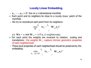
50. PCA vs Locally Linear Embedding
[Saul, L. K., & Roweis, S. T. (2000).
embedding.]
50
An introduction to locally linear

51. 51
Multi-dimensional scaling
• Input:
– An m × m dissimilarity matrix d, where d(i, j) is the distance between
instances xi and xj
– Desired dimension k of the embedding.
• Output:
– Coordinates zi ∈ Rk for each instance i that minimize a “stress”
function quantifying the mismatch between distances as given by d
and distances of the data representation in Rk.

52. Stress functions
• Common stress functions include:
– The least-squares or Kruskal-Shephard criterion:
m
L L
i=1 jI=i
– The Sammon mapping:
(d(i, j) − lzi j
− z l) 2
m
L L
i=1 jI=i
(d(i, j) − lzi j
− z l) 2
d(i, j)
52
,
which emphasizes getting small distances correct.
• Gradient-based optimization is usually used to find zi

53. 53
Other dimensionality reduction methods
• Independent component analysis (ICA)
• More generally: factor analysis
• Local linear embeddings (LLE)
• Neighborhood component analysis (NCA)
• ...
• Some methods do dimensionality reduction jointly with a supervised
learning task, or a set of such tasks

54. A generalizing perspective
Y1 Y2 YD
X1 XK

• Let Y
5
be observed data and X be hidden (latent) variables or factors
that generate the data
• The goal is to find how many such variables there are, and the model
through which they generate the data
conditional
• E.g. Mixture models: K hidden variables, Gaussian
distributions
• E.g. PCA: K hidden variables, Gaussian models
• E.g. ICA: K hidden variables, non-Gaussian models
5Roweis and Gharamani, 1999
54

55. Graphical models
• More generally, the data (yellow circles) can be generated by a more
complex structure.
• We can model all variables and their interactions using a graph structure
• Local probabilistic models describe how neighbours influence each other
• The overall model represents a joint probability distribution over all
variables (observed and latent)
55

56. 56
More generally: Autoencoders
• We have some data and try to learn a latent variable space that explains it
• The goal is to minimize reconstruction error
• In PCA, we used squared loss - this indicates an implicit Gaussian
assumption
• More generally, from data bfy we obtain a mapping z, then we can use
an inverse mapping g to go back from z to y
• We want to maximize the likelihood of the data

57. More generally: Autoencoders
Data y
Encoder
f(.)
z z = f(y)
Decoder
g(.)
y* = g(z)
57
L = ky - g(f (y))k2
L = - log p(y|g(z))
2

58. 58
Two views of auto encoders
• We just implement functions for f , g (e.g. lots of sigmoids in layers) -
this gives rise to deep auto encoders, trained by gradient descent
• We commit to full-blow probabilistic models, treating z as probabilistic
random variable - this gives rise to variational auto encoders