Downloaded 16 times


![Matrices & Vectors
• All (almost) entities in MATLAB are matrices
• Easy to define:
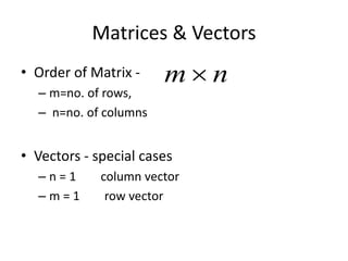
• Use ‘,’ or ‘ ’ to separate row elements
• use ‘;’ to separate rows
>> A = [1 3; 5 8]
A = 1 3
5 8
>> A = [1,3; 5,8]
A = 1 3
5 8](https://image.slidesharecdn.com/introductiontomatlab-161219072339/85/Introduction-to-matlab-7-320.jpg)
![Sequences…….
• t =1:10
t =
1 2 3 4 5 6 7 8 9 10
• k =2:-0.5:-1
k =
2 1.5 1 0.5 0 -0.5 -1
• y=[2:2:12]
y=
2 4 6 8 10 12
• B = [1:4; 5:8]
x =
1 2 3 4
5 6 7 8](https://image.slidesharecdn.com/introductiontomatlab-161219072339/85/Introduction-to-matlab-12-320.jpg)
![Matrix...
• a vector x = [1 2 5 1]
x =
1 2 5 1
• a matrix x = [1 2 3; 5 1 4; 3 2 -1]
x =
1 2 3
5 1 4
3 2 -1](https://image.slidesharecdn.com/introductiontomatlab-161219072339/85/Introduction-to-matlab-14-320.jpg)
![Matrix operations…
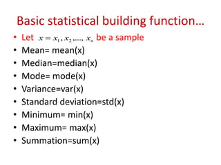
• Let A be a matrix….
• Determinant= det(A)
• Transpose= A’
• Rank = rank(A)
• Inverse= inv(A)
• Trace = trace(A)
• Eigen value=eig(A)
• Eigen value and vector= [V,D] = eig(A)
• Matrix multiplication= A*B
• Matrix multiplication= A.*B [elementwise]
• Singular values= svd(A)](https://image.slidesharecdn.com/introductiontomatlab-161219072339/85/Introduction-to-matlab-16-320.jpg)
![Cont…
• diag diagonal atrix
• triu upper triangular matrix
• tril lower triangular matri
• rand randomly generated matrix
• C=rand(5,4)
• triu(C)
• tril(C)
• diag([0.9092;0.5163;0.2661])](https://image.slidesharecdn.com/introductiontomatlab-161219072339/85/Introduction-to-matlab-17-320.jpg)

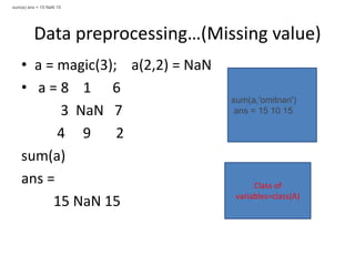
![Random number generation….
• Normal distribution:
normrnd(mu,sigma) for a single value
normrnd(mu,sigma,m,n) or
normrnd(mu,sigma[m,n]) for matrix having
m row and ncolumn
• Poisson distribution:
poissrnd(lamda)
poissrnd(lamda,m,n)
poissrnd(lamda,[m,n])
Binomial distribution:
binornd(N,P)
binornd(N,P,m,n)
binornd(N,P,[m,n])](https://image.slidesharecdn.com/introductiontomatlab-161219072339/85/Introduction-to-matlab-21-320.jpg)
![Cont…
• Geometric distribution:
geornd(p)
geornd(p,m,n)
geornd(p,[m,n])
• Beta distribution:
betarnd(A,B)
betarnd(A,B,m,n)
betarnd(A,B,[m,n])
Exponential distribution:
exprnd(mu)
exprnd(mu,m,n)
exprnd(mu,[m,n])
Gamma distribution:
gamrd(A,B)
gamrnd(A,B,m,n)
gamrnd(A,B,[m,n])](https://image.slidesharecdn.com/introductiontomatlab-161219072339/85/Introduction-to-matlab-22-320.jpg)
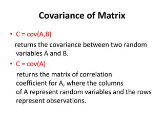
![Example…
• A = [5 0 3 7; 1 -5 7 3; 4 9 8 10];
C = cov(A)
• A = [3 6 4]; B = [7 12 -9];
cov(A,B)](https://image.slidesharecdn.com/introductiontomatlab-161219072339/85/Introduction-to-matlab-25-320.jpg)
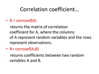
![Example…..
• x = randn(6,1);
• y = randn(6,1);
• A = [x y 2*y+3];
• R = corrcoef(A)
• A = randn(10,1);
• B = randn(10,1);
• R = corrcoef(A,B)](https://image.slidesharecdn.com/introductiontomatlab-161219072339/85/Introduction-to-matlab-27-320.jpg)
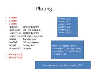
![Regression…
load moore
y=moore(:,6)
x1=ones(length(y),1)
x2=moore(:,1:5)
x=[x1 x2]
% now perform regression %
[b,bint,r,rint,stats]=regress(y,x)](https://image.slidesharecdn.com/introductiontomatlab-161219072339/85/Introduction-to-matlab-29-320.jpg)
![Test…
• %Single mean test
load stockreturns
x = stocks(:,3)
length(x)
[h,p,ci,stats] = ttest(x)
load stockreturns
x = stocks(:,3);
h = ttest(x,0,0.01)
• %paired mean test
load examgrades
x = grades(:,1);
y = grades(:,2);
[h,p] = ttest(x,y)](https://image.slidesharecdn.com/introductiontomatlab-161219072339/85/Introduction-to-matlab-30-320.jpg)
![Cont…
%paired mean test
load examgrades
x = grades(:,1);
y = grades(:,2);
[h,p] = ttest2(x,y)
load examgrades
x = grades(:,1);
y = grades(:,2);
[h,p] = ttest(x,y,0.01)
Similar way F-test , z-test, chi-square test etc
%t-Test for a Hypothesized Mean
load examgrades
x = grades(:,1);
h = ttest(x,75)
%One-Sided t-Test
load examgrades
x = grades(:,1);
h = ttest(x,65,'right')](https://image.slidesharecdn.com/introductiontomatlab-161219072339/85/Introduction-to-matlab-31-320.jpg)
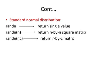
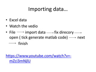
![ANOVA…
% ANOVA one way
y = meshgrid(1:5);
y = y + normrnd(0,1,5,5)
p = anova1(y)
%ANOVA two way........
load popcorn
popcorn
[p,tbl] = anova2(popcorn,3);](https://image.slidesharecdn.com/introductiontomatlab-161219072339/85/Introduction-to-matlab-32-320.jpg)


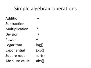
This document provides an introduction to MATLAB. It discusses that MATLAB is a high-level language for technical computing where everything is a matrix and it is easy to perform linear algebra. It describes the MATLAB desktop interface and valid variable names. It also summarizes how to perform basic operations like addition, subtraction, multiplication, etc. on matrices and vectors. Finally, it outlines various matrix operations, statistical functions, random number generation, and plotting in MATLAB.